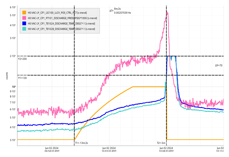
Monthly FAMIS Check (#26490)
Note: This is my first time I have run the scripts for these in O4. So I opened up the scripts to make sure there were no excitations to bump H1 out of Observing. Probably complete coincidence, but when I opened the T240 script via gedit, H1 had a lockloss! (I had Verbal running at the time on NoMachine session.) I'm sure it wasn't me, but just making a note. :)
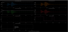
T240 Centering Script Output:
Averaging Mass Centering channels for 10 [sec] ...
2024-06-03 08:44:03.268450
There are 15 T240 proof masses out of range ( > 0.3 [V] )!
ETMX T240 2 DOF X/U = -0.461 [V]
ETMX T240 2 DOF Y/V = -0.33 [V]
ETMX T240 2 DOF Z/W = -0.395 [V]
ITMX T240 1 DOF X/U = -1.271 [V]
ITMX T240 1 DOF Y/V = 0.346 [V]
ITMX T240 1 DOF Z/W = 0.453 [V]
ITMX T240 3 DOF X/U = -1.315 [V]
ITMY T240 3 DOF X/U = -0.597 [V]
ITMY T240 3 DOF Z/W = -1.671 [V]
BS T240 1 DOF Y/V = -0.363 [V]
BS T240 3 DOF Y/V = -0.311 [V]
BS T240 3 DOF Z/W = -0.454 [V]
HAM8 1 DOF X/U = -0.332 [V]
HAM8 1 DOF Y/V = -0.427 [V]
HAM8 1 DOF Z/W = -0.706 [V]
All other proof masses are within range ( < 0.3 [V] ):
ETMX T240 1 DOF X/U = -0.113 [V]
ETMX T240 1 DOF Y/V = -0.078 [V]
ETMX T240 1 DOF Z/W = -0.123 [V]
ETMX T240 3 DOF X/U = -0.067 [V]
ETMX T240 3 DOF Y/V = -0.202 [V]
ETMX T240 3 DOF Z/W = -0.065 [V]
ETMY T240 1 DOF X/U = 0.062 [V]
ETMY T240 1 DOF Y/V = 0.094 [V]
ETMY T240 1 DOF Z/W = 0.164 [V]
ETMY T240 2 DOF X/U = -0.09 [V]
ETMY T240 2 DOF Y/V = 0.165 [V]
ETMY T240 2 DOF Z/W = 0.08 [V]
ETMY T240 3 DOF X/U = 0.178 [V]
ETMY T240 3 DOF Y/V = 0.087 [V]
ETMY T240 3 DOF Z/W = 0.101 [V]
ITMX T240 2 DOF X/U = 0.151 [V]
ITMX T240 2 DOF Y/V = 0.256 [V]
ITMX T240 2 DOF Z/W = 0.248 [V]
ITMX T240 3 DOF Y/V = 0.149 [V]
ITMX T240 3 DOF Z/W = 0.136 [V]
ITMY T240 1 DOF X/U = 0.084 [V]
ITMY T240 1 DOF Y/V = 0.1 [V]
ITMY T240 1 DOF Z/W = 0.005 [V]
ITMY T240 2 DOF X/U = 0.07 [V]
ITMY T240 2 DOF Y/V = 0.237 [V]
ITMY T240 2 DOF Z/W = 0.091 [V]
ITMY T240 3 DOF Y/V = 0.063 [V]
BS T240 1 DOF X/U = -0.165 [V]
BS T240 1 DOF Z/W = 0.132 [V]
BS T240 2 DOF X/U = -0.067 [V]
BS T240 2 DOF Y/V = 0.05 [V]
BS T240 2 DOF Z/W = -0.113 [V]
BS T240 3 DOF X/U = -0.156 [V]
Assessment complete.
STS Centering Script Output:
Averaging Mass Centering channels for 10 [sec] ...
2024-06-03 09:03:13.267069
There are 2 STS proof masses out of range ( > 2.0 [V] )!
STS EY DOF X/U = -4.047 [V]
STS EY DOF Z/W = 2.792 [V]
All other proof masses are within range ( < 2.0 [V] ):
STS A DOF X/U = -0.496 [V]
STS A DOF Y/V = -0.709 [V]
STS A DOF Z/W = -0.681 [V]
STS B DOF X/U = 0.376 [V]
STS B DOF Y/V = 0.958 [V]
STS B DOF Z/W = -0.456 [V]
STS C DOF X/U = -0.655 [V]
STS C DOF Y/V = 0.886 [V]
STS C DOF Z/W = 0.356 [V]
STS EX DOF X/U = -0.06 [V]
STS EX DOF Y/V = 0.011 [V]
STS EX DOF Z/W = 0.051 [V]
STS EY DOF Y/V = 0.048 [V]
STS FC DOF X/U = 0.244 [V]
STS FC DOF Y/V = -1.03 [V]
STS FC DOF Z/W = 0.667 [V]
Assessment complete.
