patrick.thomas@LIGO.ORG - posted 15:01, Wednesday 14 February 2024 (75860)
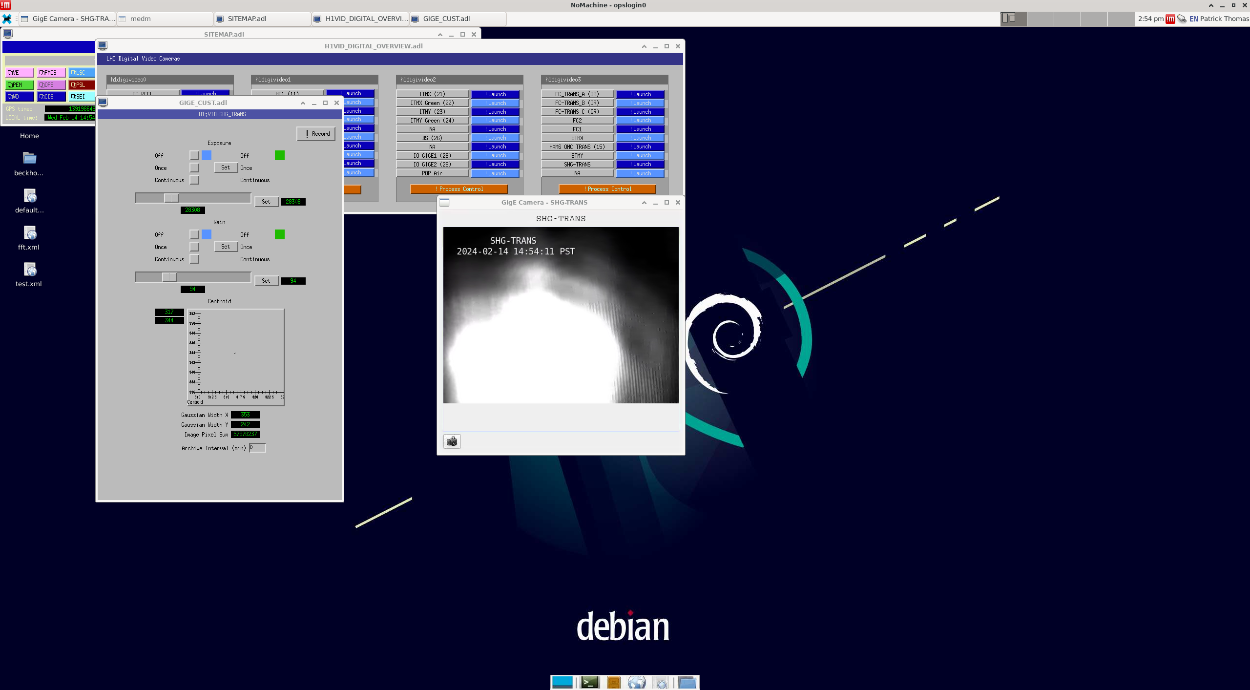
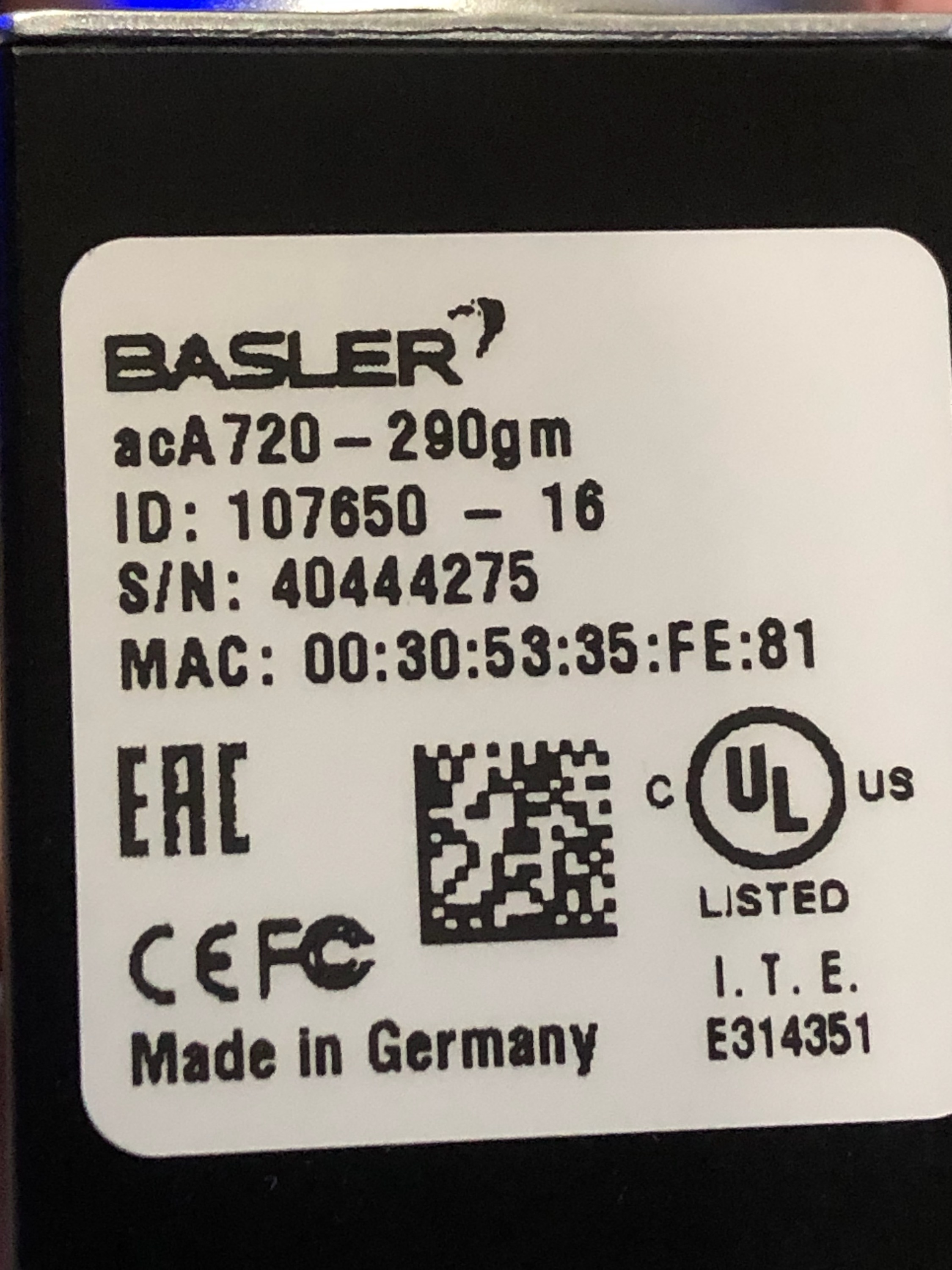
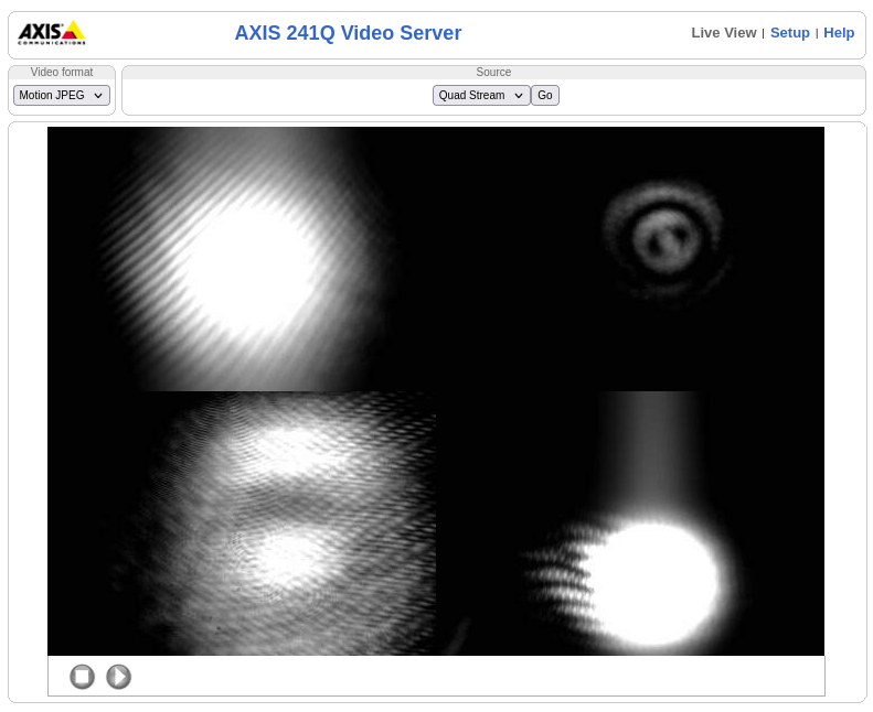
Added SHG TRANS camera to h1digivideo3
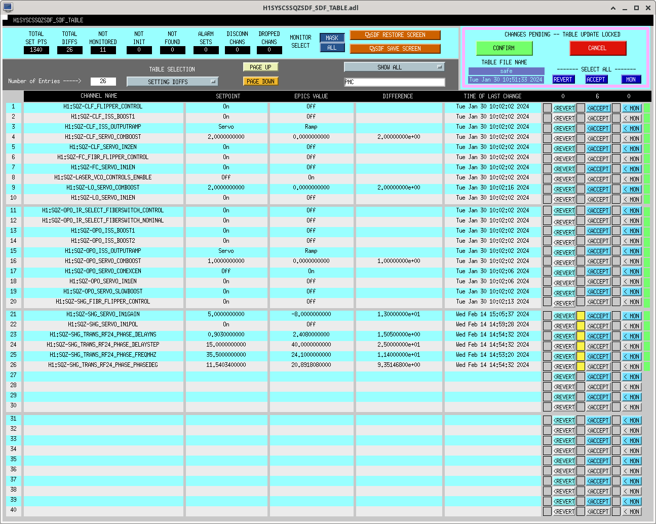
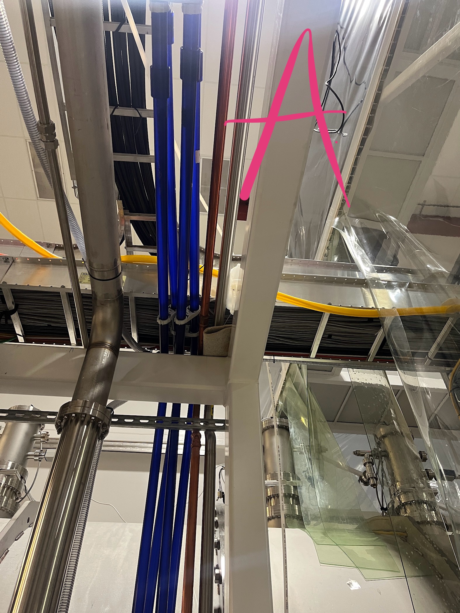
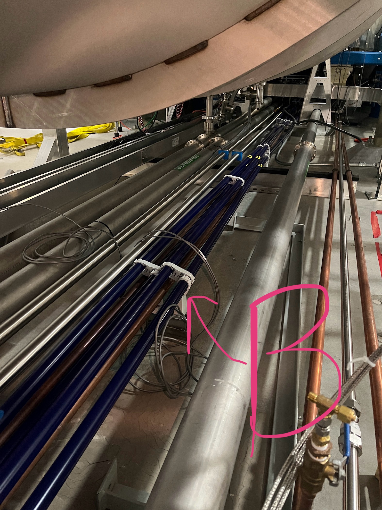
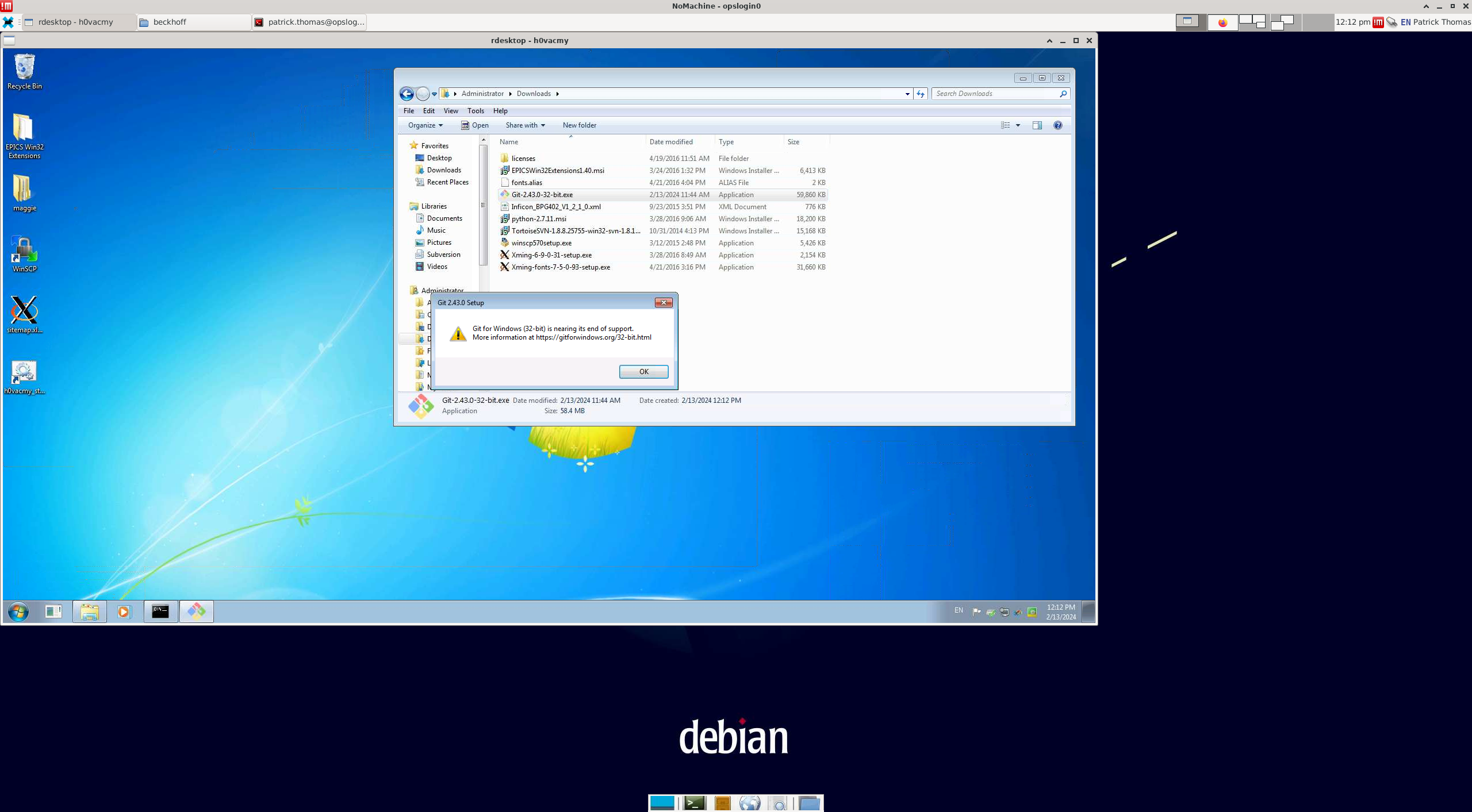
Dave, Richard, Filiberto, Tony, Daniel, Patrick


Added to puppet for h1digivideo3 and to MEDM. See attached images. I'm a little worried about the load on this machine, the IOC for this camera has started printing gstreamer queue overrun messages.
Images attached to this report