Camilla, Naoki

To find the optimal ADF demod phase for ADF servo, we scanned the ADF demod phase with ADF servo running, without SQZ ASC. The command to scan we used is as follows. We scanned the ADF demod phase from 72 to 92 deg. +2 deg and 120s delay time for each step, 10 steps in total.

ezcastep H1:SQZ-ADF_OMC_TRANS_PHASE -s '120' '+2,10'

The attached figure shows that the nominal ADF demod phase of 80 deg is already optimal value. So we left the ADF demod phase as it is.

TITLE: 12/09 Eve Shift: 00:00-08:00 UTC (16:00-00:00 PST), all times posted in UTC
STATE of H1: Commissioning
OUTGOING OPERATOR: Ryan C
CURRENT ENVIRONMENT:
    SEI_ENV state: CALM
    Wind: 4mph Gusts, 2mph 5min avg
    Primary useism: 0.05 μm/s
    Secondary useism: 0.65 μm/s
QUICK SUMMARY:

Detector Locked for 2hrs45mins, and we are in Commissioning for the next ~15minutes.

Sheila, Elenna, Camilla. Last done in August 72140. Doing now as BRUCO shows ASC coherences 74664 and want to understand current ASC coupling beofre OM2 commissioning.

Saved in /ligo/gitcommon/NoiseBudget/aligoNB/aligoNB/H1/couplings/

The new CHARD_Y quiet time reference of H1:ASC-CHARD_Y_SM was very different to the old quiet time reference: compare new (red) to 10th August (blue) of bottom left plot attached.

TITLE: 12/08 Day Shift: 16:00-00:00 UTC (08:00-16:00 PST), all times posted in UTC
STATE of H1: Commissioning
INCOMING OPERATOR: Oli
SHIFT SUMMARY:

16:47UTC Robert went into the CER to turn on an AC and he turned it back on at 17:03UTC and off again at 17:18UTV

I updated ITMY mode8s setting in lscparams after confirming the settings work in a few locks, FM1+FM5+FM10 G= +0.1. ISC_LOCK and VIOLIN_DAMPING. I'm still leaving ITMYs 5/6s gain set to zero as I'm not totally confident in the settings yet, it seems to be damping mode6 but slowly ringing up mode5.

19:08UTC Lockloss

Each of the arms went through increase flashes twice and I had to intervene to find DIFF IR and again during PRMI locking, there were no flashes so I tapped PRM in yaw based on the AS AIR camera. Lockloss at OFFLOAD_DRMI_ASC

I changed the SEI_CONF to microseism before the next lock acquisition attempt

20:03 UTC DIFF IR was not able to lock, complaining of "Bad Xarm alignmen" and I looked at the Xarm error signals and they were indeed quite bad so I took us down to start an IA

20:25 UTC during MICH_BRIGHT there were BS saturations which is unusual and it was not able to make it through the state, it was due to a poor BS alignment. I adjusted the BS in pitch by almost a microradian and the camera looked much better and IA was able to continue

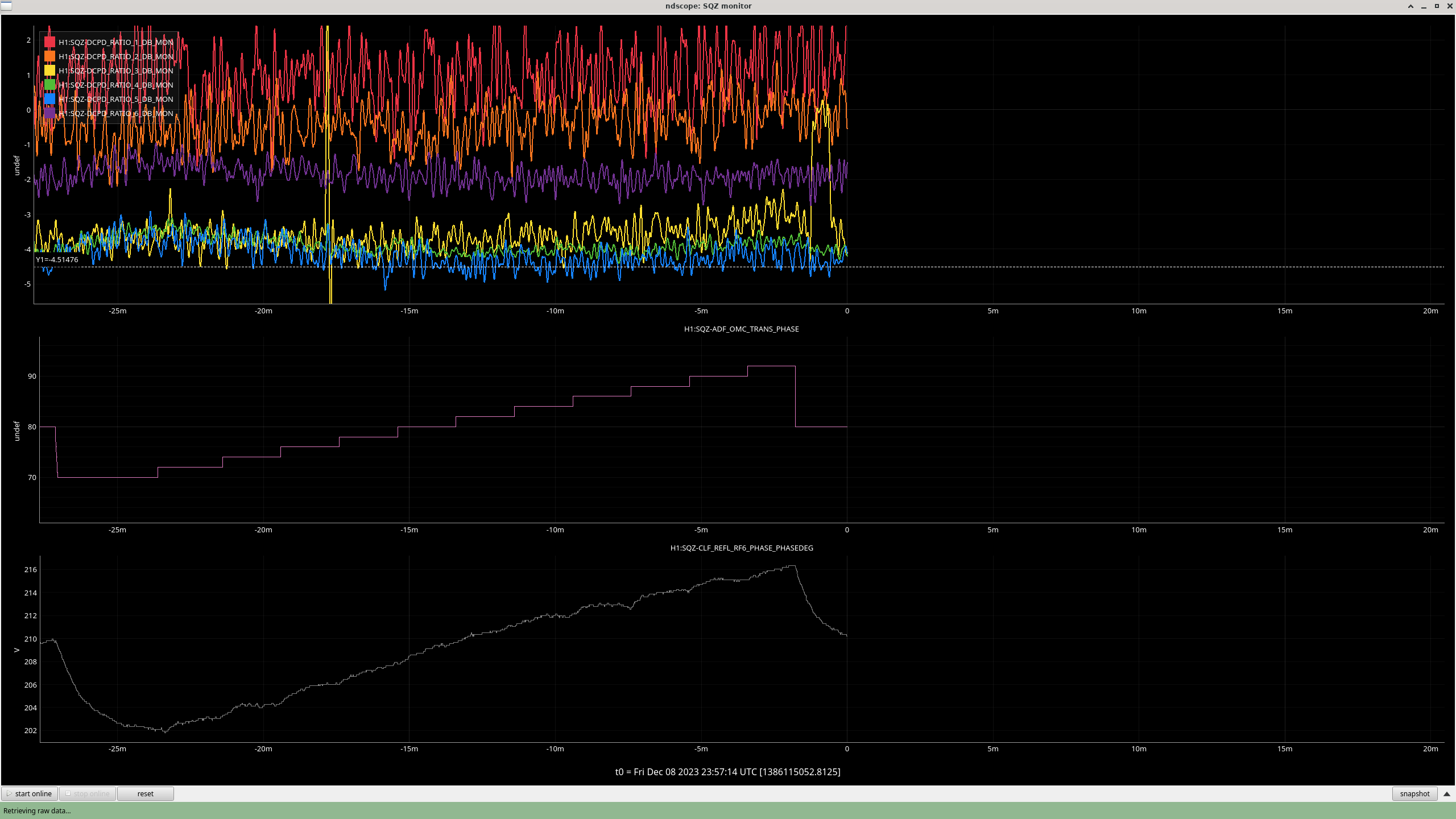
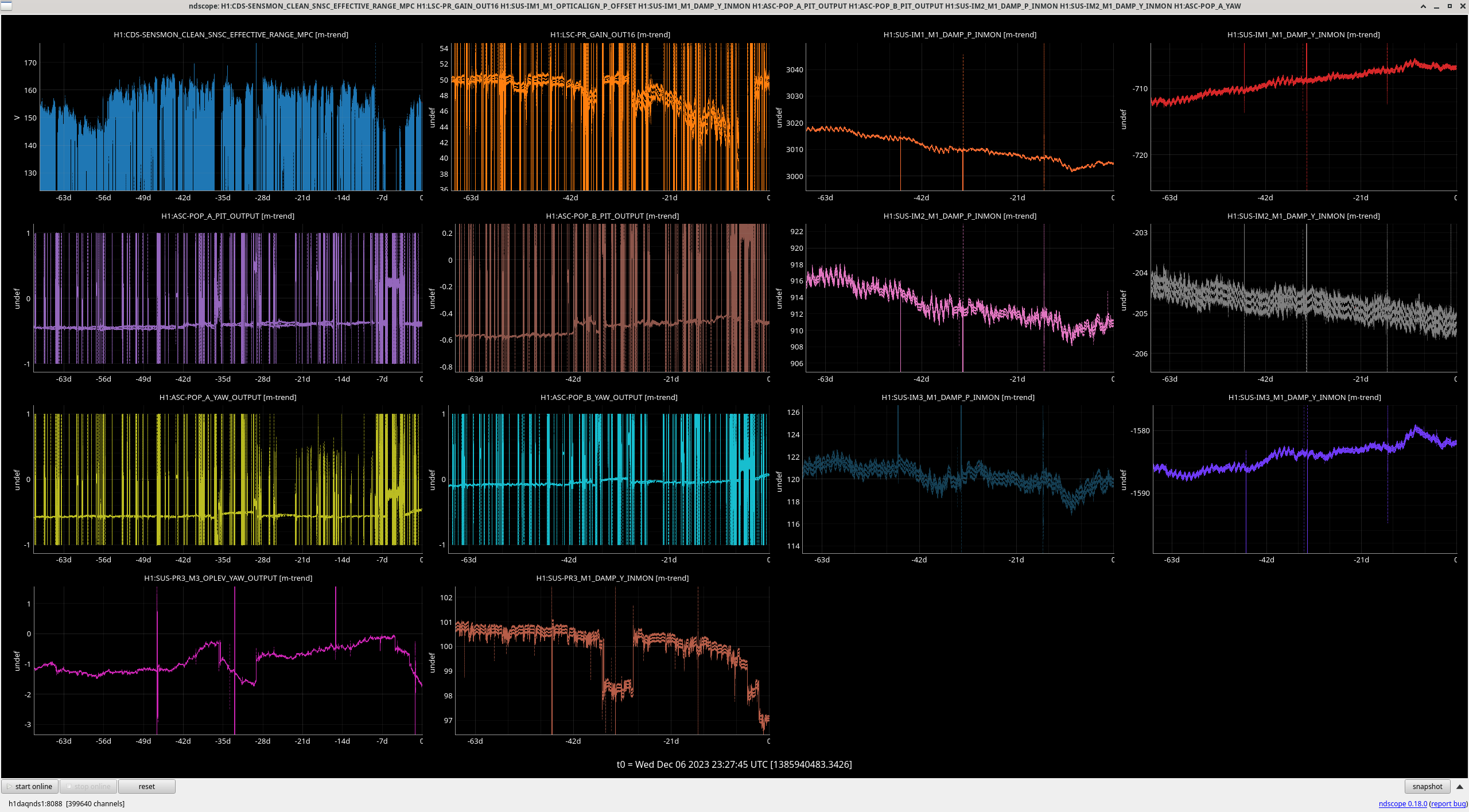
21:26 back to NLN and we started commissioning at 21:30UTC, after relocking DARM was still dominated by the ~508Hz oscillation from ITMY modes5/6 as seen in the LL.

I wasn't really able to damp ITMY mode5/6, all the settings I tried would only damp 1 while ringing up the other, I tried +/- gain with 30 degrees of phase

LOG:                                                                                                                                                                                                                                                                                                                                                             

Naoki, Sheila, Camilla

We changed the sqzparms use_ifo_as42_asc flag to False for this lock to watch SQZ without IFO ASC now we have the sqz angle feedback 74485. FC ASC left on. Not accepting the sdf's as we plan turn ASC back on at the end of commissioning.

Closes FAMIS 26221

Laser Status:
    NPRO output power is 1.819W (nominal ~2W)
    AMP1 output power is 67.9W (nominal ~70W)
    AMP2 output power is 136.7W (nominal 135-140W)
    NPRO watchdog is GREEN
    AMP1 watchdog is GREEN
    AMP2 watchdog is GREEN

PMC:
    It has been locked 2 days, 0 hr 31 minutes
    Reflected power = 16.23W
    Transmitted power = 109.8W
    PowerSum = 126.0W

FSS:
    It has been locked for 0 days 0 hr and 45 min
    TPD[V] = 0.9395V

ISS:
    The diffracted power is around 2.4%
    Last saturation event was 0 days 0 hours and 46 minutes ago

Possible Issues: None

EX sat then lockloss

Last night I turned off the CER ACs, that were again producing the 13.1 Hz broad comb in DARM (we had shut these down before: https://alog.ligo-wa.caltech.edu/aLOG/index.php?callRep=73430), for two hours to see if the frequency would be changed when I turned them back on. It did, but by this morning the AC peak had drifted back to 13.1 Hz and was again producing peaks in DARM. I think we can run with these three of six shut off - we will monitor the temperature today and leave them off if there are no problems. The figure shows the spectra associated with the 2 or 3 Mpc improvement, even at these very high microseisms.

16:47 UTC off

17:03 on

17: 18 off

Fri Dec 08 10:11:32 2023 INFO: Fill completed in 11min 28secs

Jordan confirmed a good fill curbside.

TITLE: 12/08 Day Shift: 16:00-00:00 UTC (08:00-16:00 PST), all times posted in UTC
STATE of H1: Observing at 156Mpc
OUTGOING OPERATOR: Austin
CURRENT ENVIRONMENT:
    SEI_ENV state: SEISMON_ALERT
    Wind: 9mph Gusts, 8mph 5min avg
    Primary useism: 0.06 μm/s
    Secondary useism: 0.58 μm/s
QUICK SUMMARY:

• We've been locked for 13:20, in observing since 02:37UTC
• CDS reports 12 channels not connecting, they're all MONITOR_NUC26 channels
• Microseism still higher than usual
• ITMY modes 5/6 and 8 are decently high, ~4.5 on the VIOLIN_MONITOR medm, I'll work to damp these down

TITLE: 12/08 Eve Shift: 00:00-08:00 UTC (16:00-00:00 PST), all times posted in UTC
STATE of H1: Observing at 155Mpc
INCOMING OPERATOR: Austin
SHIFT SUMMARY:

Decent evening shift even with several earthquakes rolling through (there is another M5.6 New Caledonia eq about 10min away now!).  L1 has been down for most of this shift due to a power outtage.
LOG:

• 0033-0035 Turning OFF 1 bank (or 3 AC Units) 
  • 0219-0220  Turning them back ON
• 0123 Lockloss from M5.8 Solomon Island EQ
• 0625 GRB-short (H1-only Observing)

Have had (2) south Pacific earthquakes the first half of the shift, lockloss from the first one (M5.8, Solomon Islands) and rode through the 2nd one (M5.4, Tonga).

LLO is currently recovering from a power outtage.

Jenne, TJ, Sheila, Naoki,

We looked at some trends together of what's been happening with H1's range, PRG, and various sensors related to the PRC over the last few months. 

The first screenshot here shows some of these trends, with the first horizontal cursor showing, Oct 24th a day when we had a particularly good BNS range just above 160 Mpc.  The vertical cursors are set to show a reference of what the various signals were on that good day.  Some things to notice:

• The PR3 yaw moves from Friday (74535) and Monday (74578) seem to have restored our PRG to nearly 50, with a similar stability to what we had in late October.  These moves improved our range and glitch rate, but the range is still lower than our best times in October and early November.
• The top mass osems aren't a reliable way to track PR3 yaw (neither is the optical lever): We had previously seen that PR3's optical lever wasn't tracking long term drifts well at all, (70008) so on Nov 7th we used the top mass osems to reset PR3 yaw to previous times (74065), as marked by the red arrow.  You can see that from this time forward the PRG dropped, became more noisy, and seems to drift more.  So it seems that this move started to introduce clipping probably in the LSC POP path.
• The POP QPDs also can't be used to track this shift:   POP A is the QPD used in DRMI ASC, which has large offsets applied.  Both POP A and POP B yaw would indicate that our recent moves Friday and Monday went in the wrong direction, but we observe that these moves reduced clipping in the POP LSC path (74586 and 74582).  Also, looking at their trends over the last few months they don't seem related to changes in PRG, (for example, POP A YAW was the same as at the good time in our worst PRG times 14-7 days ago). 
• Jenne suggested looking at trends of IM1-3, which are uncontrolled and could be drifting.  The second attachment shows their trends, they seem to be drfiting in a way that might correlate with outdoor temp, like many things do.  I believe these are fairly small shifts of the IMs (I'm not sure that these are calibrated into urad, for historical reasons some channels which are calibrated on other suspensions aren't calibrated in the same way on the IMs). I'm not sure that we can tell without taking some steps on some of these if they are responsible for the PRG change. 

Dana, Sheila

I plotted how the DCPD matrix has changed over the last eight years in the attached figure (DCPD_sums_and_nulls_8years). I've also included zoomed in snapshots of all the major changes within this time span with the dates and times shown (changes 1-7 attached below). For each one of these jumps in the matrix values, I checked the alogs for that day and attached any potentially relevant ones explaining what was going on at the time below:

change 1 (1) (2)

changes 2 & 3 (1) (2)

change 4 (1)

change 5 (1) (2)

change 6 (1)

change 7 (1) (2) (3) (4) (5)

Today I took "unbiased" OLGs of DHARD P and CHARD P (see 67187 for discussion of unbiased measurements and methods). Craig previously measured these loops at 60W input power before I did some additional redesign of the loops (68698, 67488, 67518).

I have plotted the open loop gain with error shading in the attached plots. You can find the measurement templates, exported data, and processing code in '/ligo/home/elenna.capote/ARM_ASC/{DHARD,CHARD}'.

The templates for the these measurements are also saved in [userapps]/asc/h1/templates/{DHARD,CHARD} as '{DHARD,CHARD}_P_olg_broadband_shaped.xml'.

CHARD P has a UGF of 3 Hz with a phase margin of 33 deg. DHARD P has a UGF of 3.4 Hz with a phase margin of 27 deg.

DHARD has two other UGFs at 1.6 Hz and 2.4 Hz. CHARD has additional UGFs around 2.5 Hz, 1.2 Hz, 0.95 Hz and 0.65 Hz.