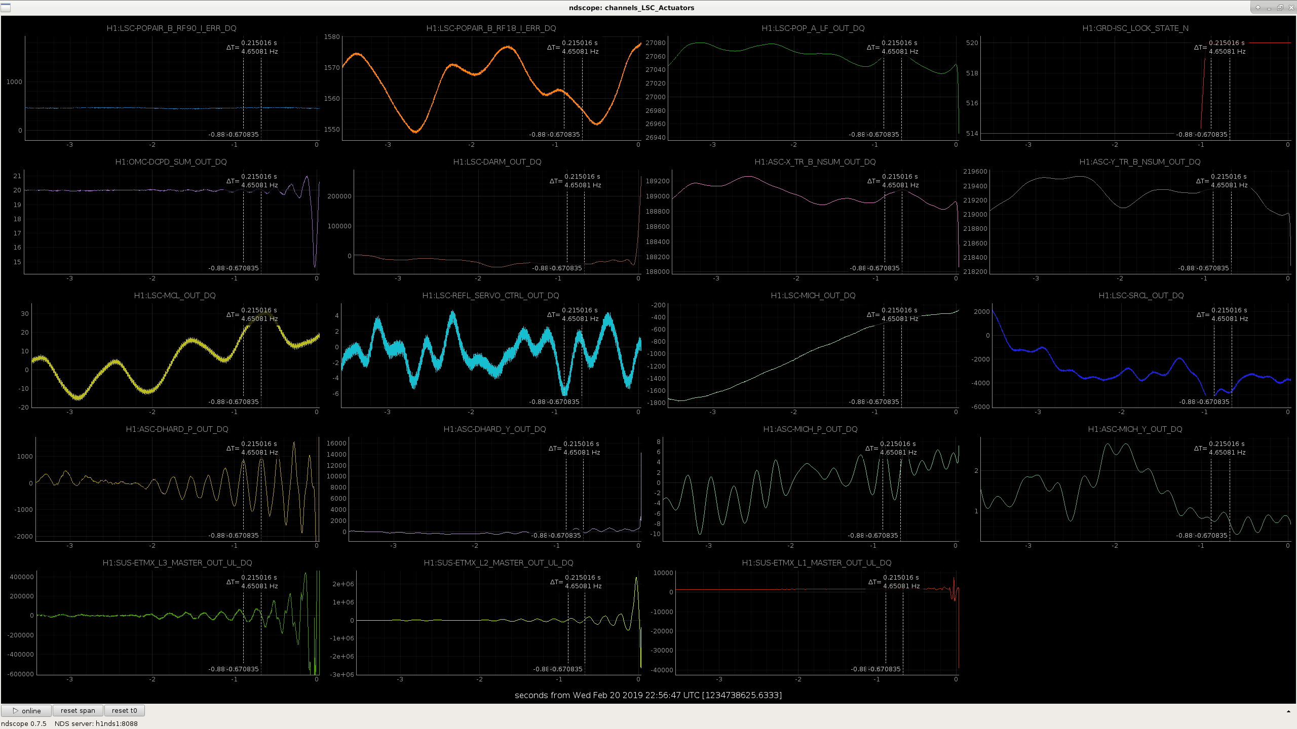
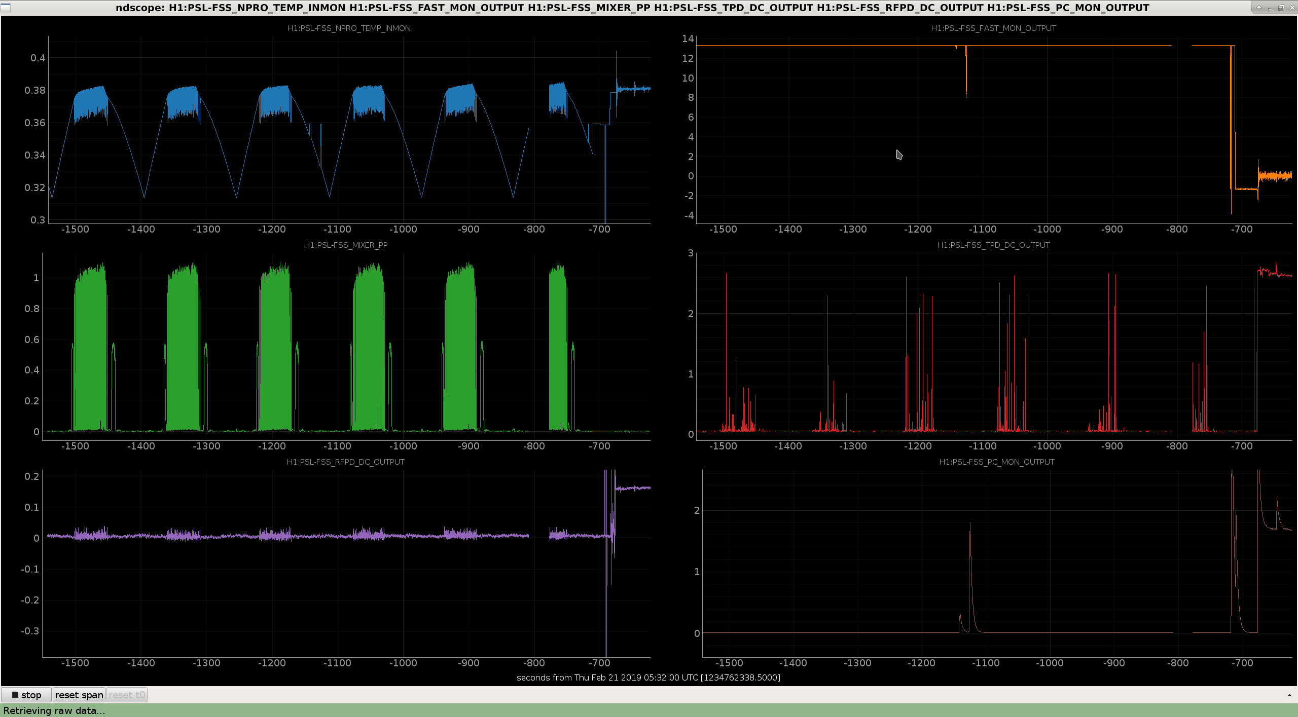
I manually locked the FSS by disabling the autolocker, moving the temperature to where it was when the FSS was previously locked, then engaging the loop. Looking at the FSS time series, it seems as though the temperature never actually reaches the top of it's range. When the FSS sees flashes, it triggers some FSS_OSCILLATION state in the PSL_FSS guardian, which ramps up and down the common gain in an attempt to unrail the PZT. It's possible that these common gain ramps were too small, happen too quickly or jerk the temperature around too quickly. I adjusted the FSS_OSCILLATION state so the gain goes down to 0 dB from 28 dB, then ramps back up. Unclear if this will actually help, probably would be smarter to tune the autolocker settings to slow things down around the flashes.
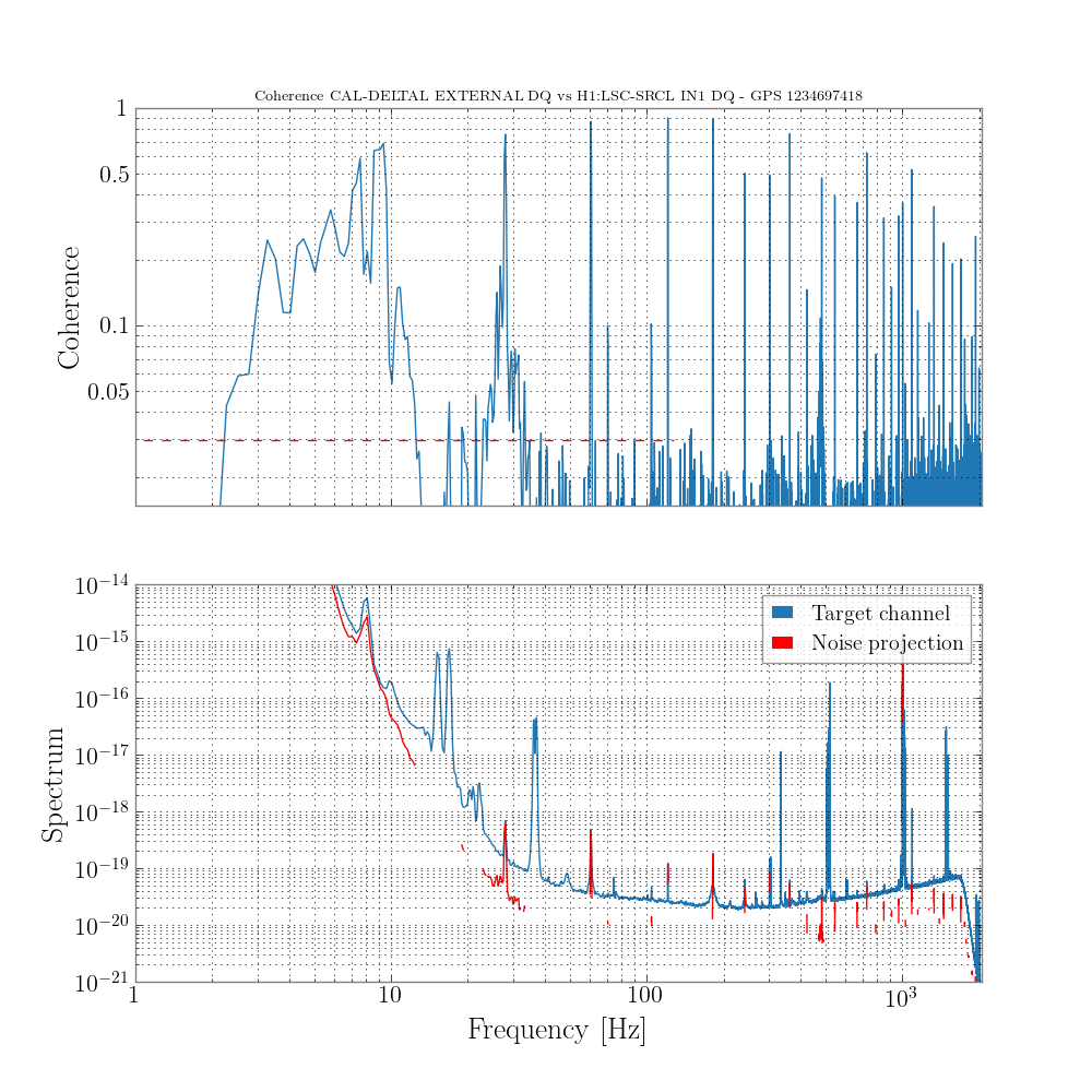
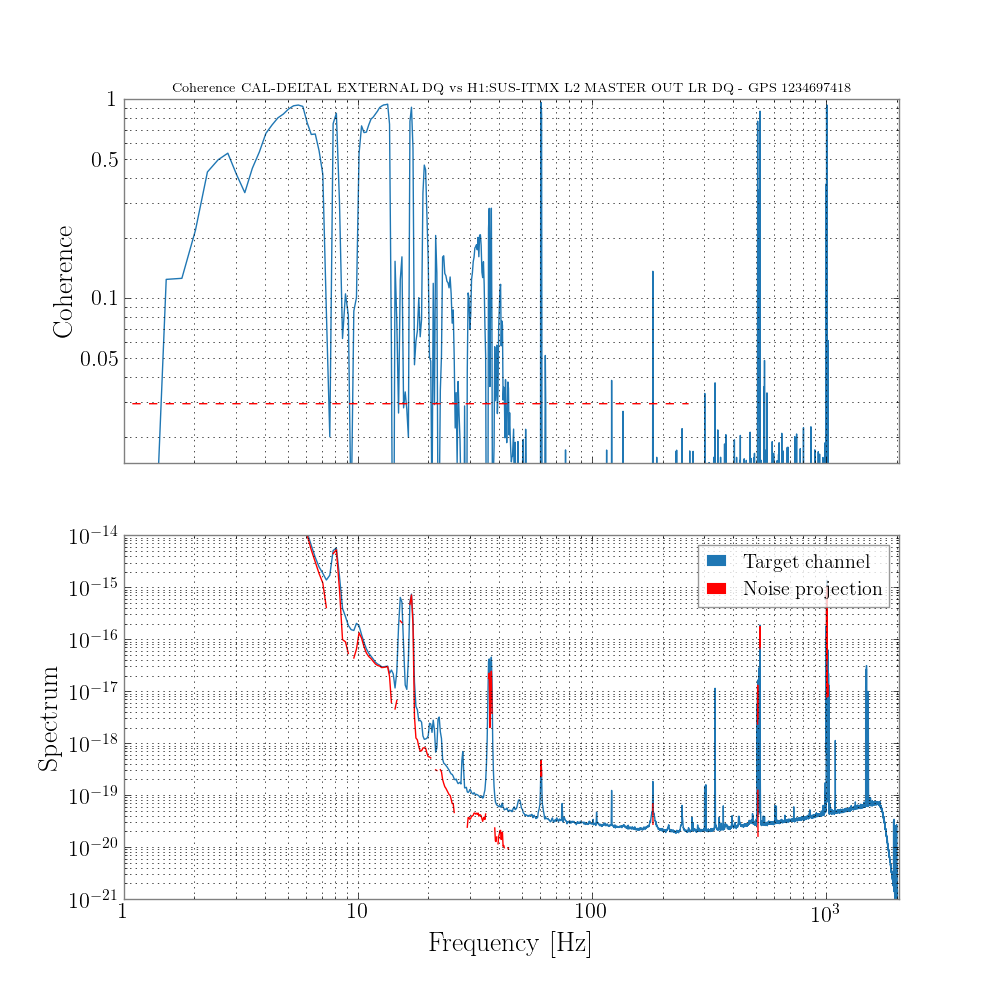
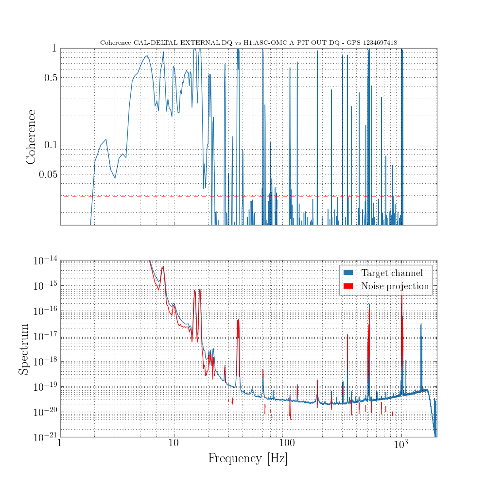
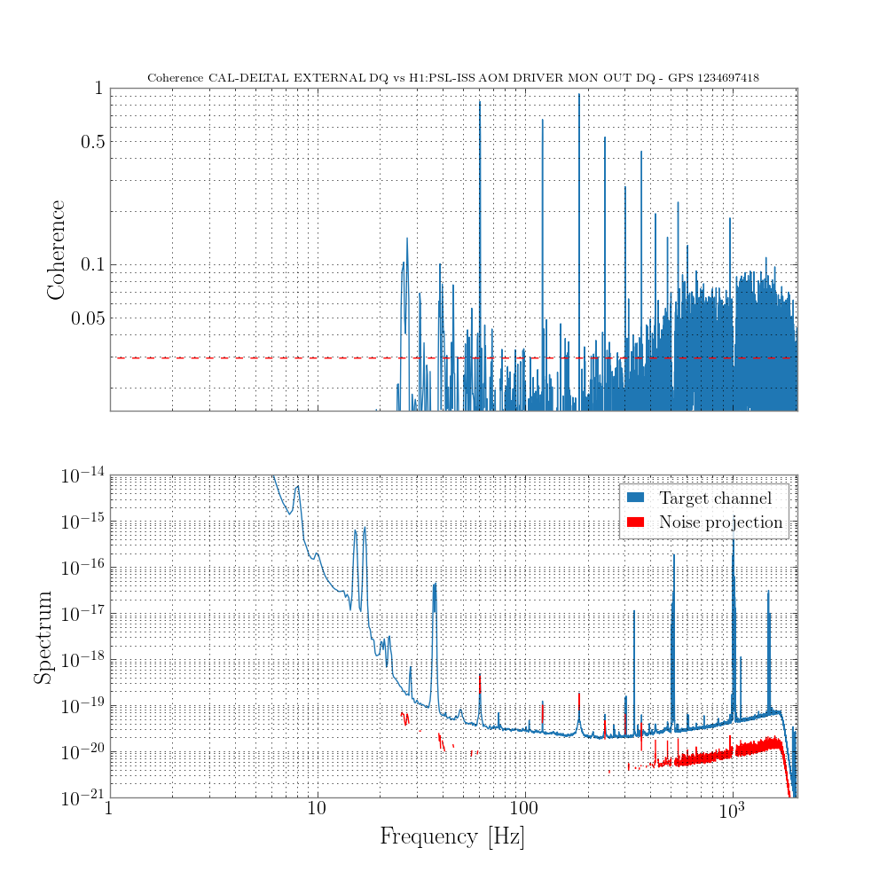
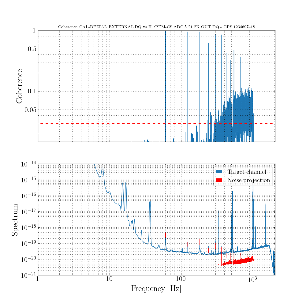
A BruCo scan for the "improved spectrum" mentioned in 47011 is available at the link below:
https://ldas-jobs.ligo.caltech.edu/~gabriele.vajente/bruco_lho_1234697418b/
I didn't use exactly the same time as in the posted spectrum, but instead used a quiet period with good range.
Some highlights:
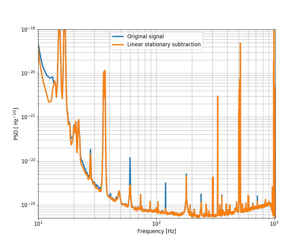
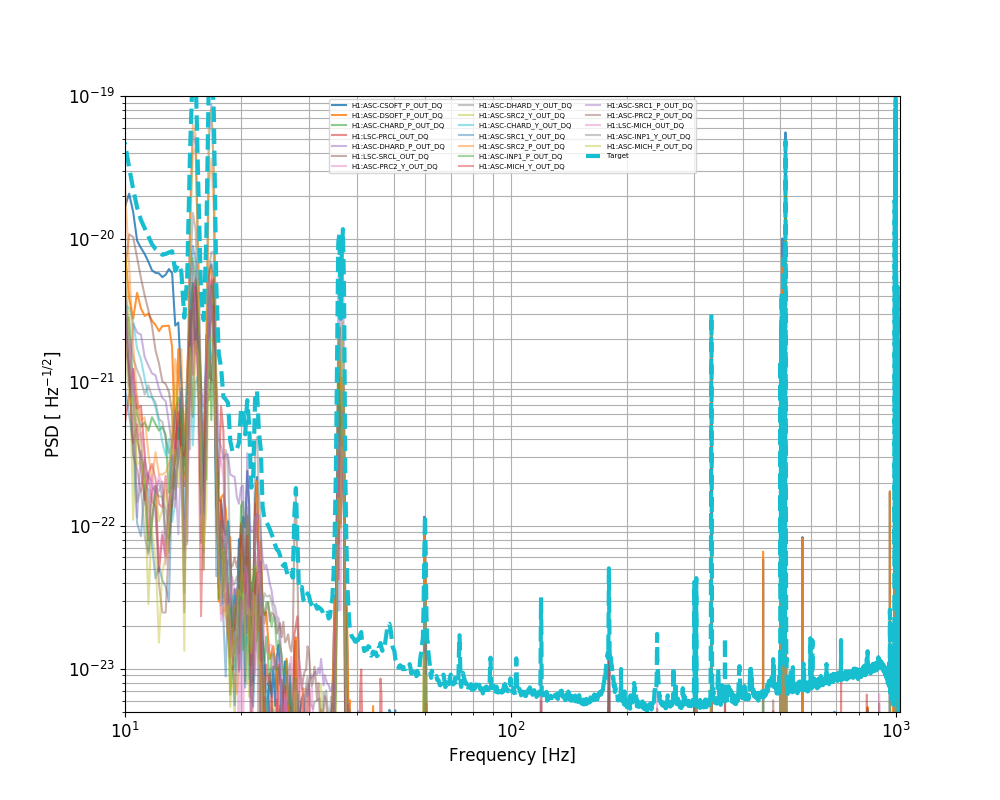
The effect of a linear noise subtraction of ASC and LSC control signals is shown below. This subtraction uses the parametric technique described in T1800552.
The coherence with ASC-OMC_RIN_OUT_DQ and similar signals is due to the fact that at low frequency the DARM noise is large enough to dominate over those signal sensing noise. This has been confirmed by taking the transfer function ASc-OMC_RIN / DARM_IN1 during a DARM injection and using it to project ASC-OMC_RIN_OUT_DQ into DARM.
Leaving Y-mid instrument-air energized until further notice.
Also ,
1415 -1445 hrs. local -> Ran HEPTA pump (testing) at Y-mid. I expect to be running this pump intermittently over the next few days for various testing purposes and will record the Start/Stops in the aLOG at the end of the day(s).
TITLE: 02/20 Day Shift: 16:00-00:00 UTC (08:00-16:00 PST), all times posted in UTC
STATE of H1: Commissioning
INCOMING OPERATOR: None
SHIFT SUMMARY:
Made it to NLN once (for a couple of minutes) & then lost lock multiple times around the LOWNOISE_ESD_ETMX step. Performed an alignment (had issues with PRC & SRC, but Jenne walked me through them).
LVEA Dust Monitor #6 is down.
LOG:
The main benefit of doing radiation pressure compensation is that we only need to handle a single suspension plant. If the plant is unchanged, we can invert it or utilizing its features in the digital control filter banks to improve the loops' noise performance.
For example, we can use optimal control techniques (specifically, the H-infinity design) to optimize the DHARD PIT loop, which enables x10 less sensing noise injection to DARM at 10 Hz yet with the same phase margin (30 deg) and a good enough residual rms level (< 1 nrad).
Please see the attached plots for details:
1. In oltf_Hinf_fit.pdf we compare the oltf using H-inf (the red trace) and the one currently used (the black trace; based on the model in LHO:46179 with a 10 W plant which seemed to match measurements done at both 10 W no RPC and at 20 W w/ RPC). The red trace has a ugf of 2.3 Hz with 30 deg phase margin (same as the black trace; the margin can be further increased if we slightly reduce the DC gain of the loop). On the other hand, the roll-off for the H-inf design is much faster than the one used currently, and it should enable about a factor of 10 more reduction of sensing noise injection to DARM in the 10-20 Hz band. At the same time, there is less phase delay at ~ 1 Hz, so the H-inf design might actually be more robust than the current filter at 1 Hz against cross-couplings.
2. We extract from the overall oltf the control filter should go into the DHARD_P filter module in ctrl_Hinf_fit.pdf. Again a comparison between how the H-inf vs. current should look like is shown in the plot.
In case people were interested in implementing it, we also provide the foton file that can be directly put into the filter in dh_p_ctrl.txt. (Only need to change the ctrl filter bank while leaving the DC gain the same, which was 30 in the model we adopted).
3. The anticipated closed-loop noise performance is shown in cl_noise_hinf_fit.pdf. The low-freq rms is ~ 0.7 nrad < 1 nrad that we need (here we assumed no reduction of input noise from the ISIFF). As a comparison, using the original loop design the rms is 0.4 nrad for the same input noise. Therefore in terms of motion stabilization the two loops should be similar. Also shown is the requirement on roll-off so that it equals to the aLIGO design noise. Here we have assumed a sensing noise of 1e-14 rad/rtHz for DHARD (LHO:46178) and an a2l coupling of 1 mm/rad.
Jenne, Hang
We also show the closed-loop response in the attached plot. The amount of gain peaking is similar for the H-inf design and the original loop.
To check the robustness of the controller, we plot the closed-loop responses with suspension plants corresponding to 8 W (blue) and 15 W of input powers. The 8 W one starts to become marginally stable but the 15 W one still seems fine. Since the RPC gain was adjusted every 2 or 3 W change of input power, and we set the gain such that it would tend to under-subtract the RP (i.e., the sus plant corresponds to input > 10 W) than over-subtract (< 10 W). The step size bounds the |error| < ~ 3 W, and the under-subtraction makes it more likely to be 12 W or 13 W. Thus the controller should be stable given the level of error likely to be happening in the RPC.
Also currently we adjust the RPC gain discretely due to lack of commissioning time. In the future the gain can be continuously/adaptively adjusted by monitoring the TR QPD sum value relative to a reference point. The gain also depends on the ASC optical response converting the digital counts back to physical angle in radians, which can be monitored with diagnostic dithering lines (low amp & @ < 10 Hz). (Also if the TCS is settled, the optical gain was generally quite stable over a lock stretch). So in the future the level of plant fluctuation should be even smaller.
[Jenne, Nutsinee]
We've added an empty state in ISC_LOCK, called INJECT_SQUEEZING. Once the SQZ automation is ready, this state should be able to tell the squeezer guardian to do the final steps for injection of squeezing.
This is an update on my previous entry 46952.
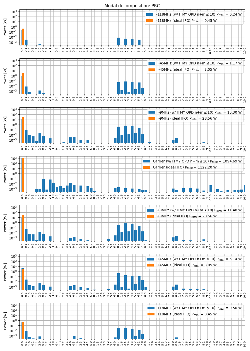
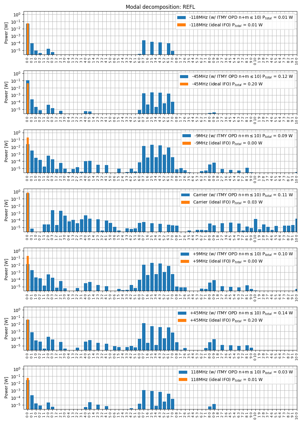
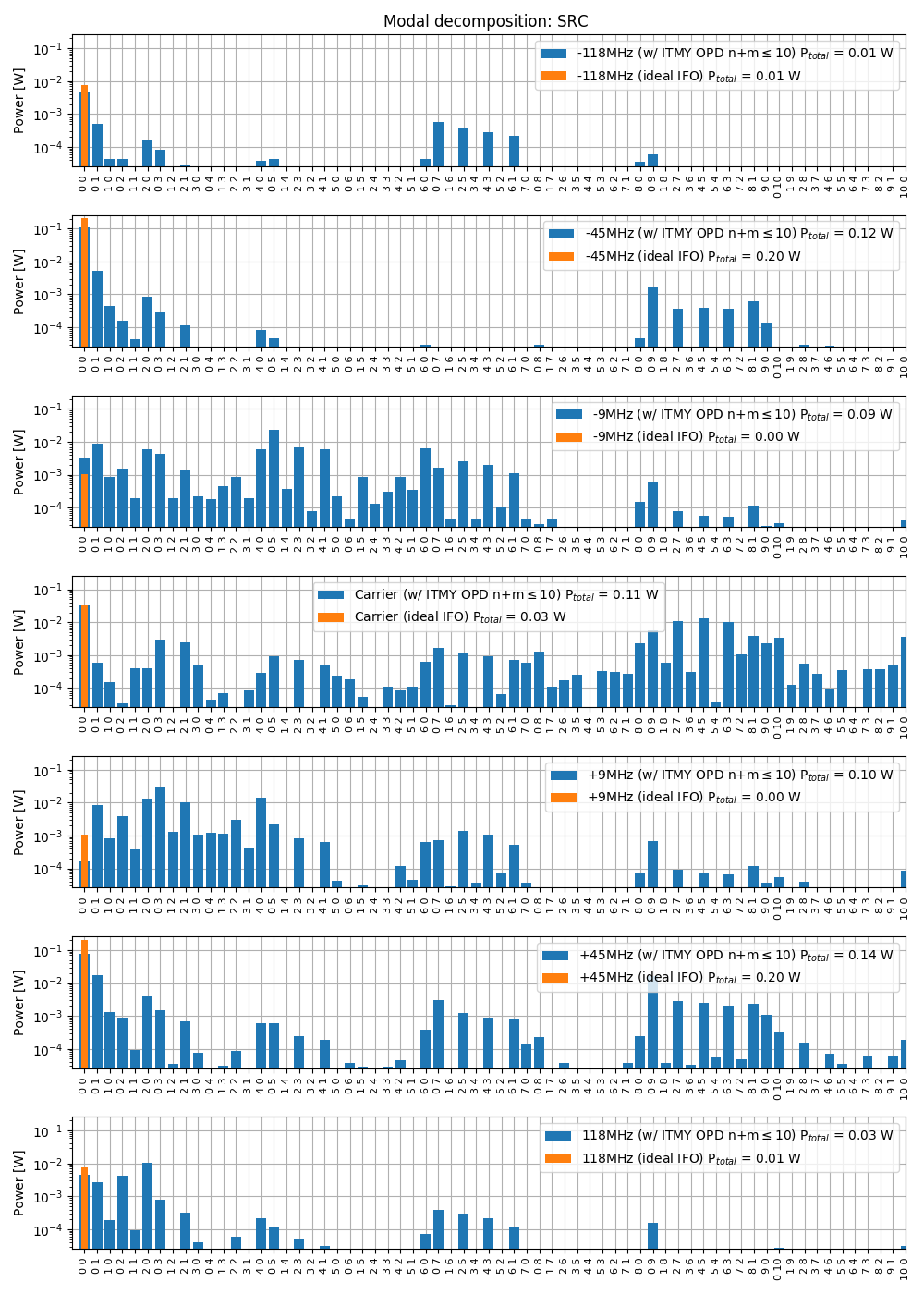
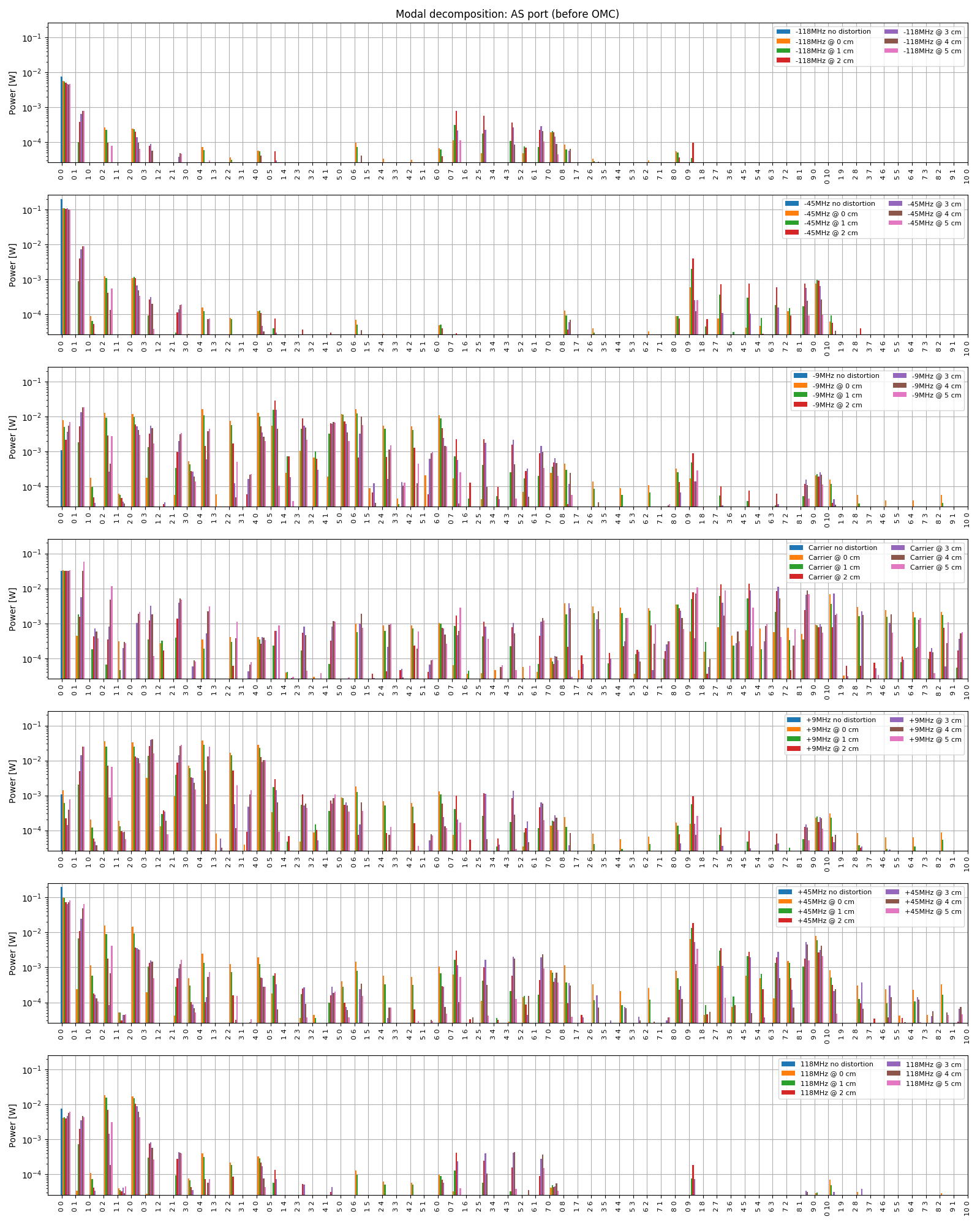
Using the optical path distortion measured by the HWS (provided by Aidan, see also 46127 and 46888) I simulated the mode content at various ports in a dual recycled Fabry-Perot Michelson interferometer. The simulation is done with MIST, using Hermite Gauss modes up to order 10, and locking the interferometer using simulated error signals. In the original entry 46952, the path distortion was about half of what we expect at 26 W (because the wavefront map provide by Aidan corresponds to a power step of about 15 W). So in the results considered here I multiplied the map by two.
Only the optical path distortion in the ITM is included, there is no deformation of the HR surface.
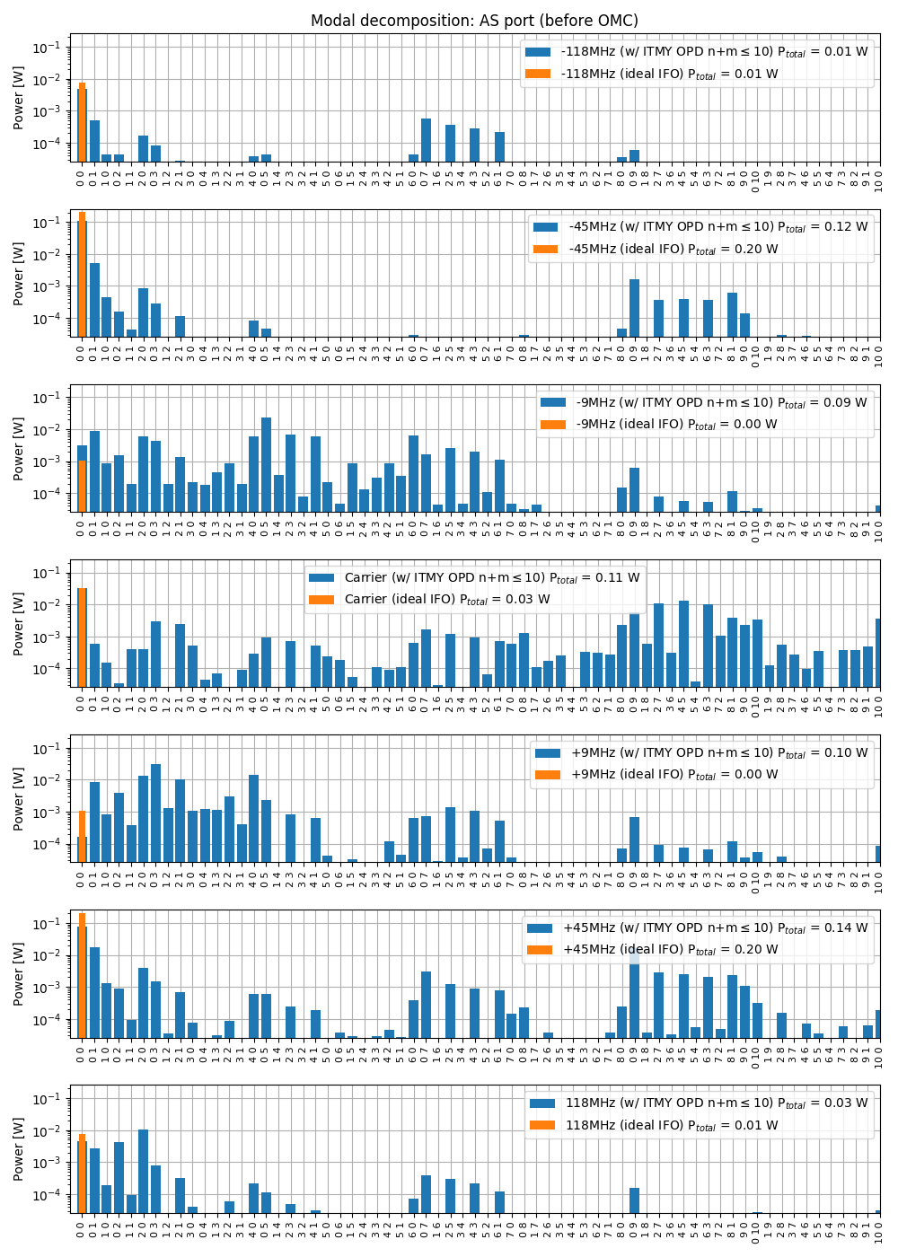
Each of the attached plots show the distribution of power into each modes, assuming 26 W of input power, 60ppm or round trip losses per arm. The orange traces are there for comparison, to show that in a ideal IFO, all power is in the fundamental TEM00 mode.
Interestingly, the point absorber seems to create some 9MHz sideband power in modes of order 9 at the AS port, which we believe are the culprit for the high RF9 modulation noise coupling.
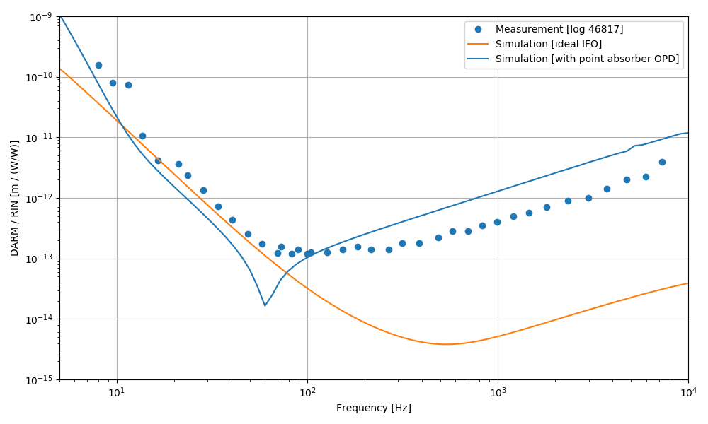
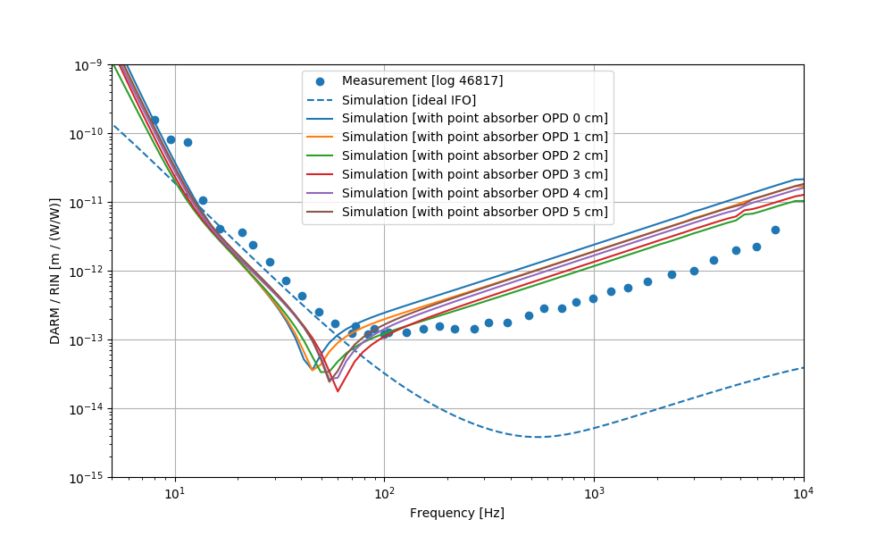
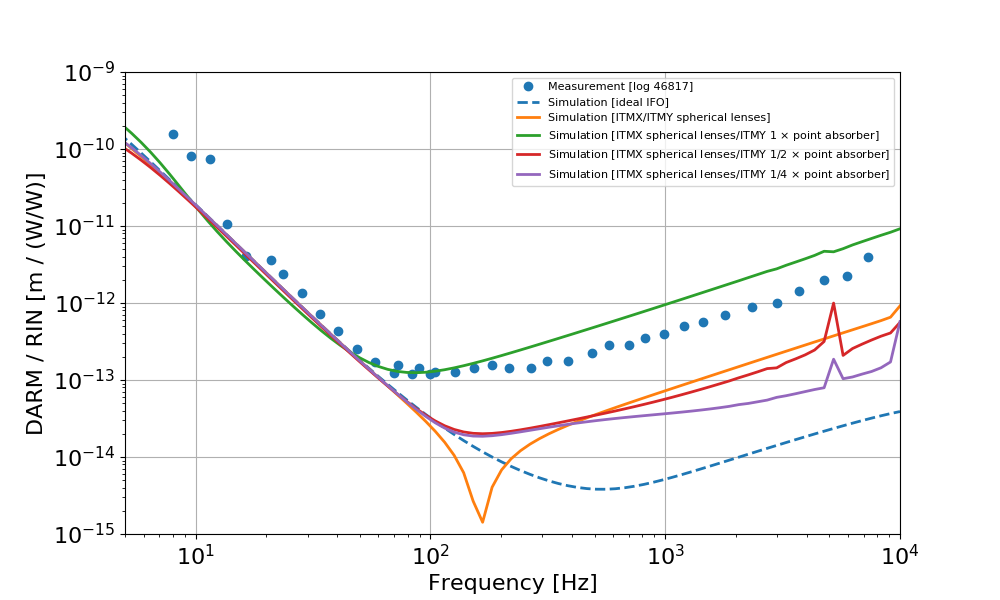
Using the same simulation described above, I could compute the coupling of input RIN to DARM. The result is shown below, compared with Craig's measurement from 46817. The distortion produced by the point absorber seems to explain qualitatively (even though not quantitatively) the increased coupling at high frequency. The magnitude of the coupling is larger in simulation, but roughly ok. The coupling scales with the amplitude of the optical path distortion, and it's likely to change if the point absorber is moved by a cm or two, probably within the uncertainty of the beam center position in the HWS map.
According to the simulation, there is about 1 mW of 9MHz sidebands power in the modes of order 9. Assuming that all of this mode is transmitted through the OMC, we can compute the DARM noise corresponding to sideband RIN:
DARM = SB_RIN * SB_POWER / (OMC_DC / DARM)
From 46985 I estimate a DARM noise at a level of DARM ~= 5e-20 m/rHz at 100 Hz. From the simulation I have OMC_DC / DARM ~= 1.2e10 W/m, from which
SB_RIN ~= 4e-7 /rHz
is the level of 9 MHz sidebands RIN that would explain the DARM noise, assuming it's all due to RF9 TEM9 mode leakage.
The position of the point absorber has, as expected, an effect on the simulation results. Here I started by centering the peak of the optical path distortion (OPD) at the center of the beam, and then move it to the side by steps os 1 cm, up to 5 cm from the center. I maintained the same peak amplitude of the OPD, so the shift does not take into account the change in the power that is actually absorbed. This simulation is just to get a feeling of how much the results change because of the uncertainty of the beam center position w.r.t. to the HWS frame.
The first plot shows that the coupling of RIN to DARM changes a bit, but not much, with the absorber position.
The second plot shows the mode content at the AS portfor the different positions. I realize this is a busy plot and hard to get much information out of it. I'll try to find a better representation soon.
CAVEAT: in all the simulations reported so far, I have included only the point absorber map on the ITMY substrate. To have a more realistic simulation, I should include the intrinsic and thermal lenses in both ITMs, as well as the effect of Ring Heaters and CO2 laser. Working on it.
Updates
In the figure below, the coupling from RIN to DARM is shown for three configurations
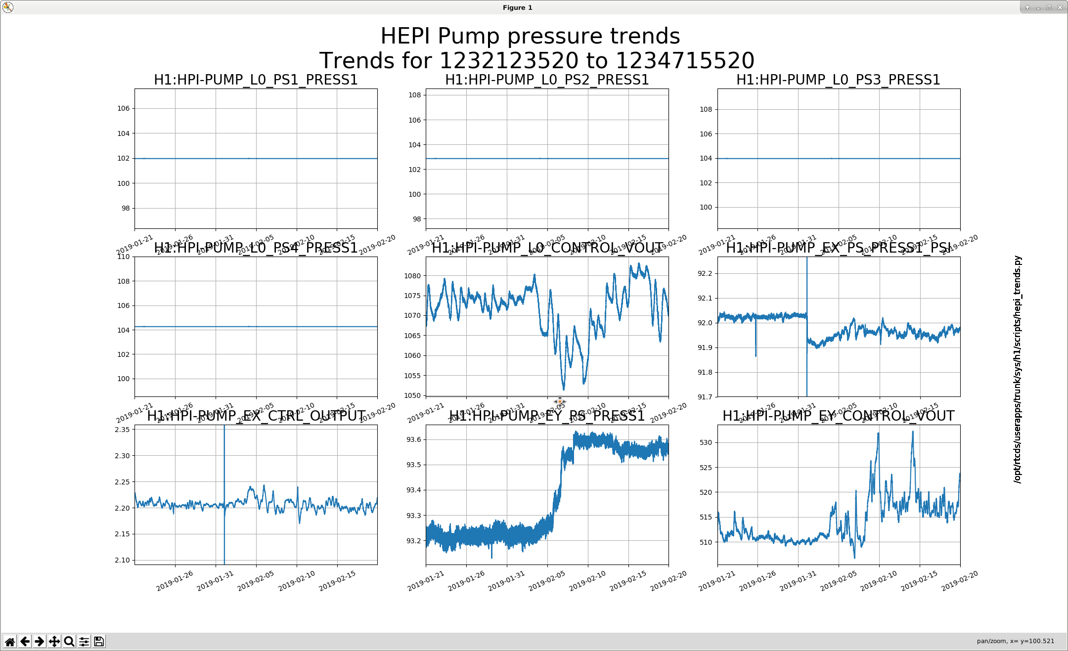
Small step in EX pressure a few weeks ago. Followed by a slightly larger step up for EY. (see attached)
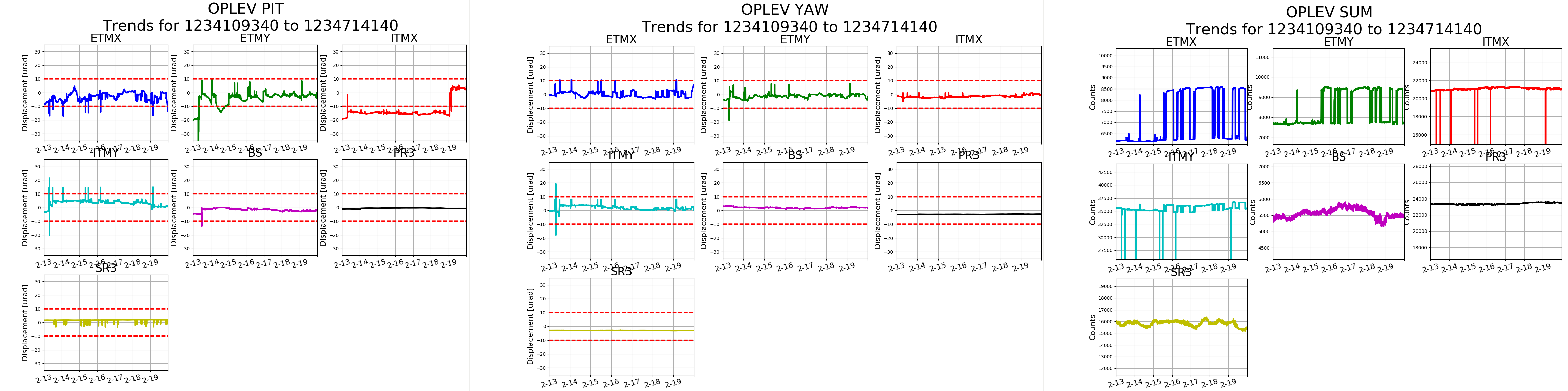
All oplevs within nominal levels (ITMx was centered yesterday during Maintenance by EdM).
There was an FSS measurement this morning; other than that No Issues to report.
Laser Status:
Front End Power is 32.46W (should be around 30 W)
70W Output Power is 70.84W
Front End Watch is GREEN
70W Watch is GREEN
PMC:
It has been locked 0 days, 1 hr 59 minutes (should be days/weeks)
Reflected power = 10.56Watts
Transmitted power = 54.41Watts
PowerSum = 64.97Watts.
FSS:
It has been locked for 0 days 0 hr and 35 min (should be days/weeks)
TPD[V] = 2.961V (min 0.9V)
ISS:
The diffracted power is around 2.2%
Last saturation event was 0 days 0 hours and 36 minutes ago (should be days/weeks)
Addressed TCS Chillers (07:50 - 8:00 AM PST today/Wed)
TITLE: 02/20 Day Shift: 16:00-00:00 UTC (08:00-16:00 PST), all times posted in UTC
STATE of H1: Commissioning
OUTGOING OPERATOR: None
CURRENT ENVIRONMENT:
Wind: 13mph Gusts, 12mph 5min avg
Primary useism: 0.05 μm/s
Secondary useism: 0.29 μm/s
QUICK SUMMARY:
Sheila, Georgia, Craig
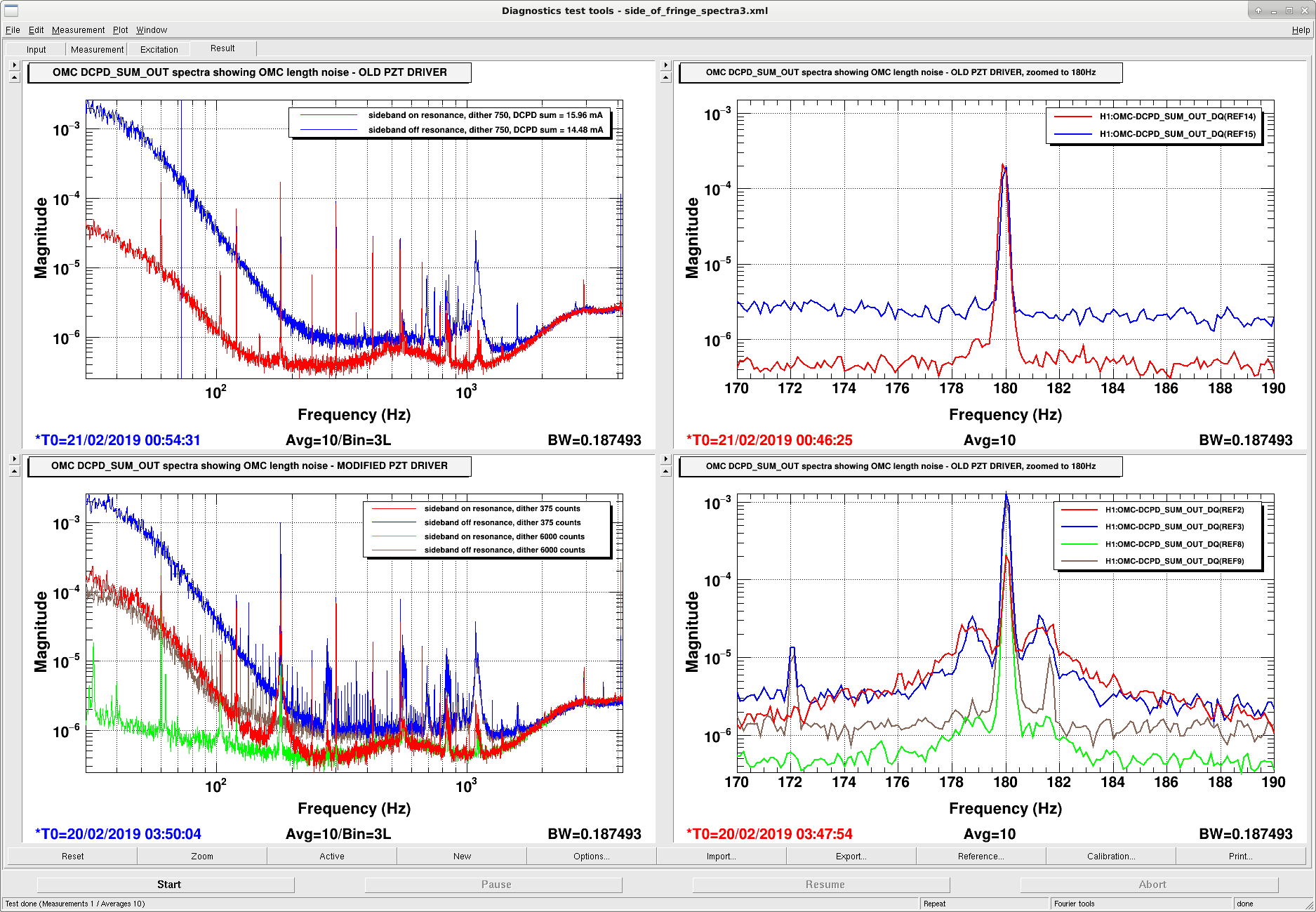
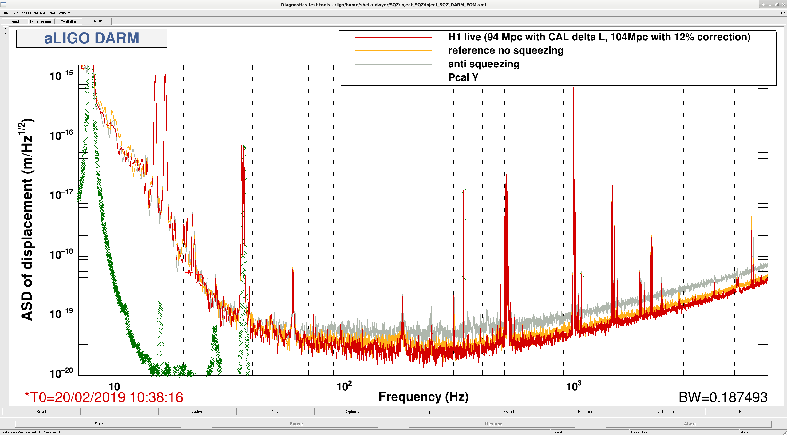
After improving the broad shoulders on the power lines by increasing the OMC dither, 47007, and finding that our 9 MHz coupling to DARM is reduced 47008 and that the DCPD cross correlation shows improved noise around 50-60Hz 47012, we decided to inject squeezing again since we know from 47006 that it can improve our sensitivity. The attached screenshot shows the reference, anti-squeezing and DARM with squeezing. The sensmon range is between 93-94Mpc, and we think that this is underestimating the range by about 12% according to the PCAL sweep that Jeff did this morning 47003.
Wonderful - very nice progress.
Great work!
Excellent news!
Great!
If it were safe to assume that the frequency dependent systematic error were the same between lock stretches (it's not), I could apply the same correction I'd done to the 2019-02-19 23:00 UTC lock stretch to this data. This is a false assumption (and, naturally, the quantification of time-dependent correct factors is back in to the realm of confusing non-functionality so I don't know *how* different parameters are), but hopefully at the ~few% level in response function change, and the effect on BNS range was mapped out in LLO:31156 to be also in the ~few% level. But y'know, because we're crazed to surpass the 100 Mpc BNS range, aka #KeepIt100, I've done the same analysis as was done in LHO:47003, multiplying the ASD at this time (Feb 20 2019 10:38:16 UTC, 1234694314, for 120 seconds) by the previous lock stretch's PCAL 2 DELTAL sweep, and computed the BNS range difference. As a testament to the hilarious comedy of life, the corrected range is 99.91 Mpc. (And note that I tried shifting the ~120 second time stretch by 15, 30 seconds on either side and the range went down to 99.5 ish, so somehow Sheila found a magically delightful time.) This ASD has not had any offline subtraction done, which I believe Team DetChar has been geared up to do. I've updated the function that generates these plots a bit, /ligo/svncommon/CalSVN/aligocalibration/trunk/Common/pyDARM correct_bns_range.py and I *know* that this function as-of-yesterday doesn't work in the control room. Regardless, I quote the exact command line used on my laptop configuration of python: python3.6 correct_bns_range.py --run='O3' --IFO='H1' --GPSstart='1234694314' --GPSend='1234694434' --PCAL2DARMTF='/ligo/svncommon/CalSVN/aligocalibration/trunk/Runs/O3/H1/Measurements/FullIFOSensingTFs/2019-02-19_H1_PCAL2DARMTF_A_PCALYRX_B_DELTALEXT_tf.txt' --PCAL2DARMCOH='/ligo/svncommon/CalSVN/aligocalibration/trunk/Runs/O3/H1/Measurements/FullIFOSensingTFs/2019-02-19_H1_PCAL2DARMTF_A_PCALYRX_B_DELTALEXT_coh.txt' --DARMmodelfile='modelparams_H1_20190219' --modelFunction='modelPars' --resultsTag='/ligo/svncommon/CalSVN/aligocalibration/trunk/Runs/O3/H1/Results/FullIFOSensingTFs/2019-02-20_H1_sensingFunction_BNSRangeCorrection' The data is committed to the CalSVN here: /ligo/svncommon/CalSVN/aligocalibration/trunk/Runs/O3/H1/Results/FullIFOSensingTFs 2019-02-20_H1_sensingFunction_BNSRangeCorrection.pdf 2019-02-20_H1_sensingFunction_BNSRangeCorrection_ASD.txt 2019-02-20_H1_sensingFunction_BNSRangeCorrection_PCAL2DELTALTF.txt
At the time of our excellent spectrum, the offline noise subtraction codes from DetChar (TJ Massenger & Derek Davis) and Calibration (Aaron Viets) gives us about 1.5 more Mpc, so we can say that we really did get above 100 Mpc - in fact about 101.4 Mpc. See, for example, a comparison of cleaned vs. pre-cleaned spectra: https://ldas-jobs.ligo.caltech.edu/~aaron.viets/H1_CAL_NoiseSub_20190220/H1_1234694144_1234698240_spectrum_comparison.png
Sheila, Nutsinee
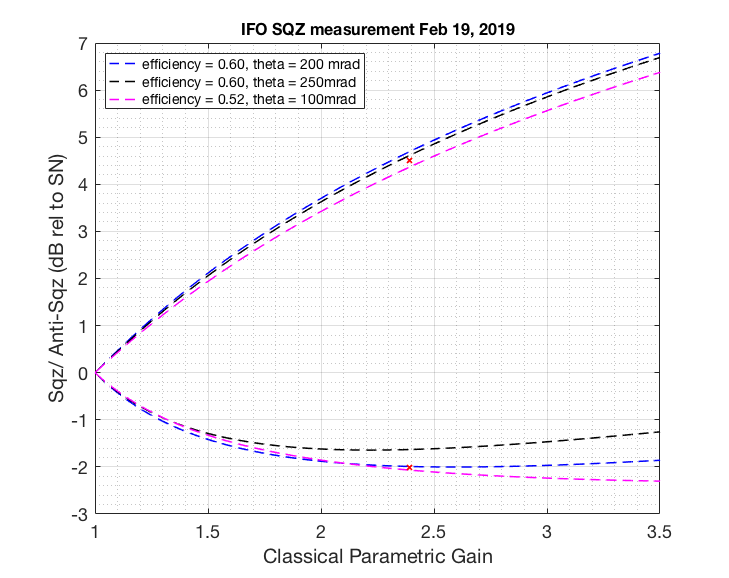
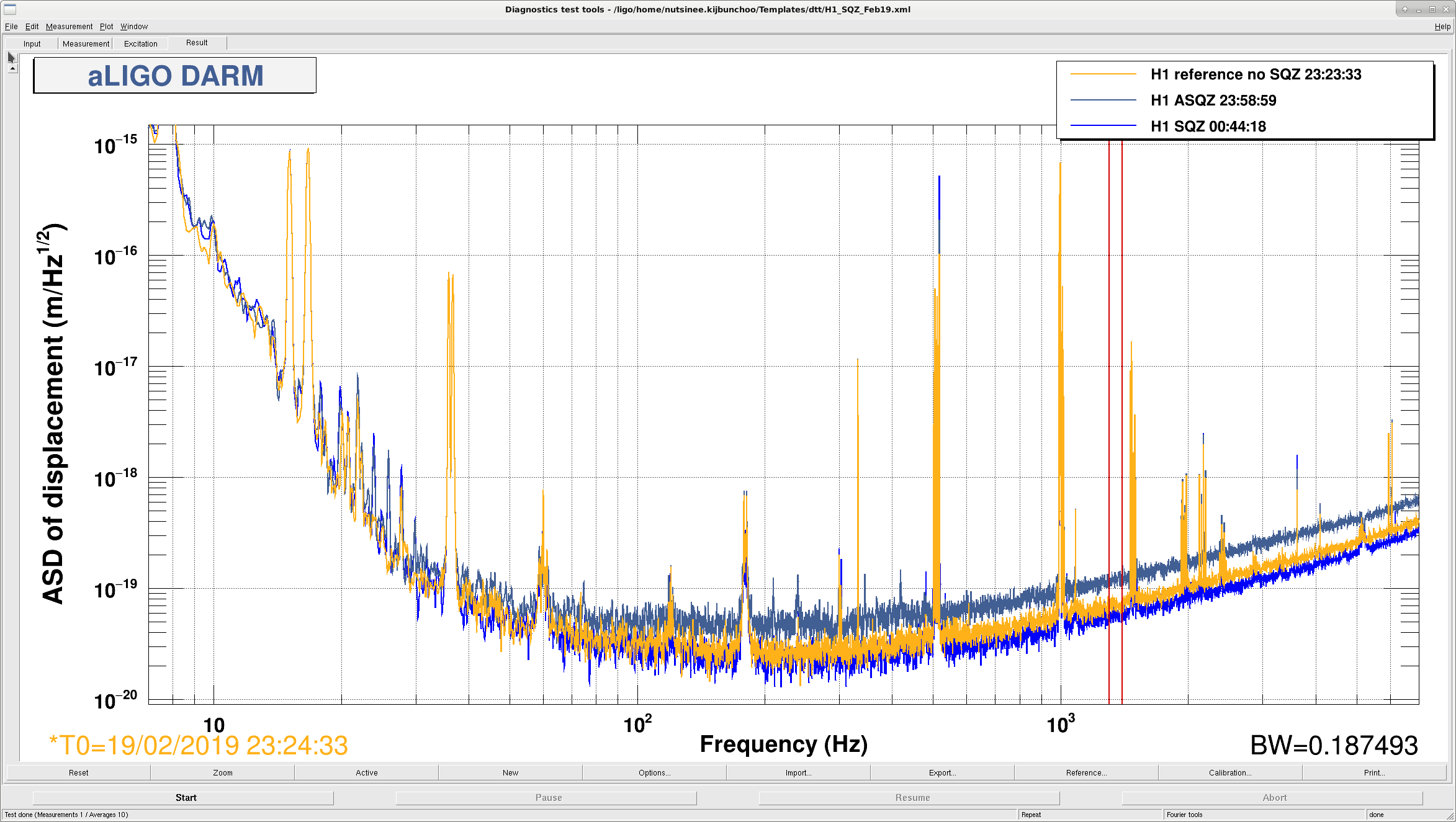
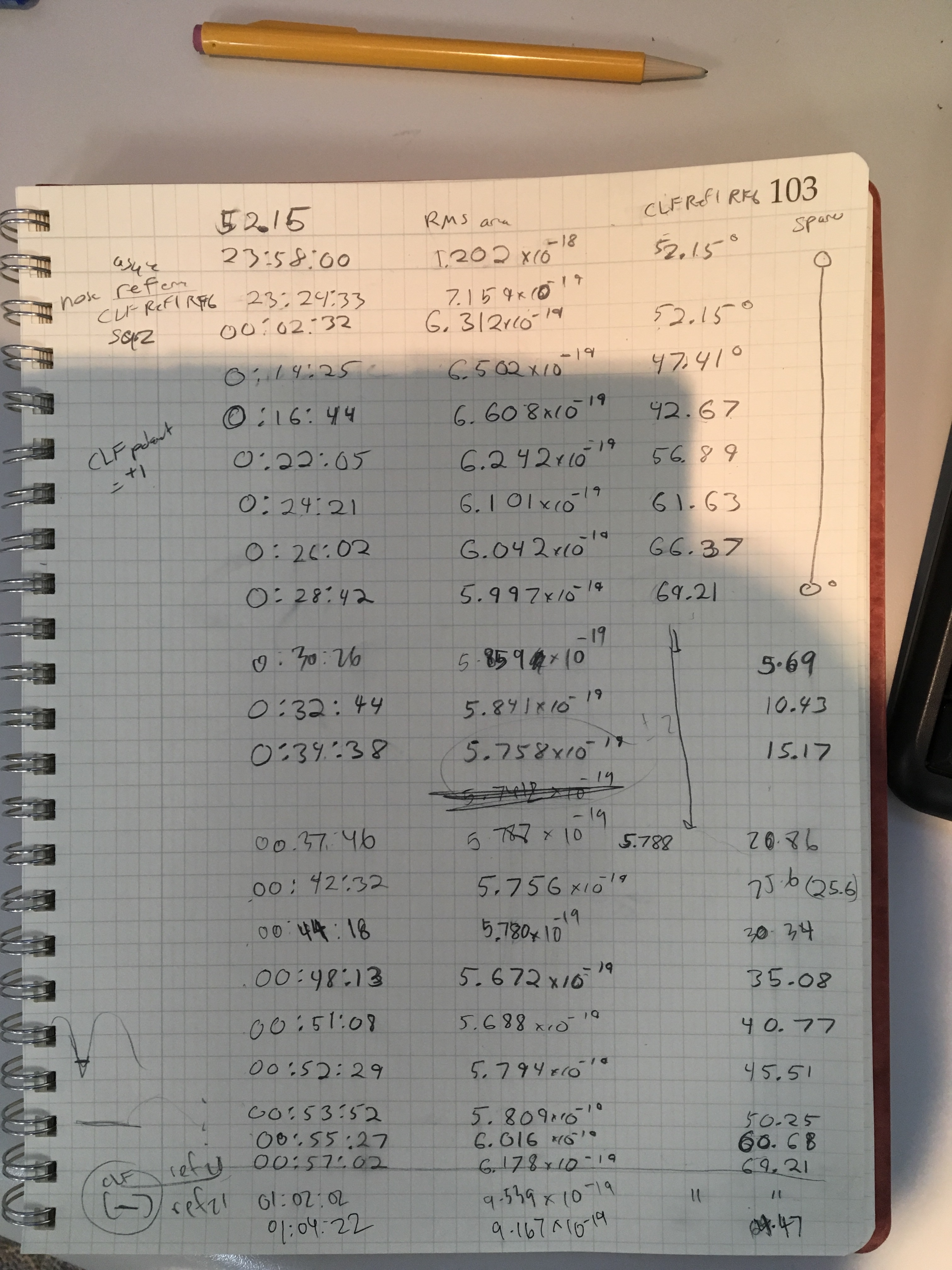
Today we took our time to carefully map out phase vs. amount of squeezing we get. Turned out the best squeezing can't simply be judged by looking at QMON (although I believe this works for asqz). In the end we were able to get 2.02 dB of sqz and 4.5 dB of asqz at a nonlinear gain of 2.39. This measurement still indicates a significant amount of loss. Optimizing the CFL phase is probably what helped the phase noise here. We think we could be limited by some technical noise (to be calculated). But attached below a usual sqz/asqz fit. It seems like our loss is approximately the same as last time (30-40%, alog46814) with better phase noise. We also got a little more RF3 today (-14.7dBm compared to -15.5 dBm last time). We used the same amount of CLF power as last time.

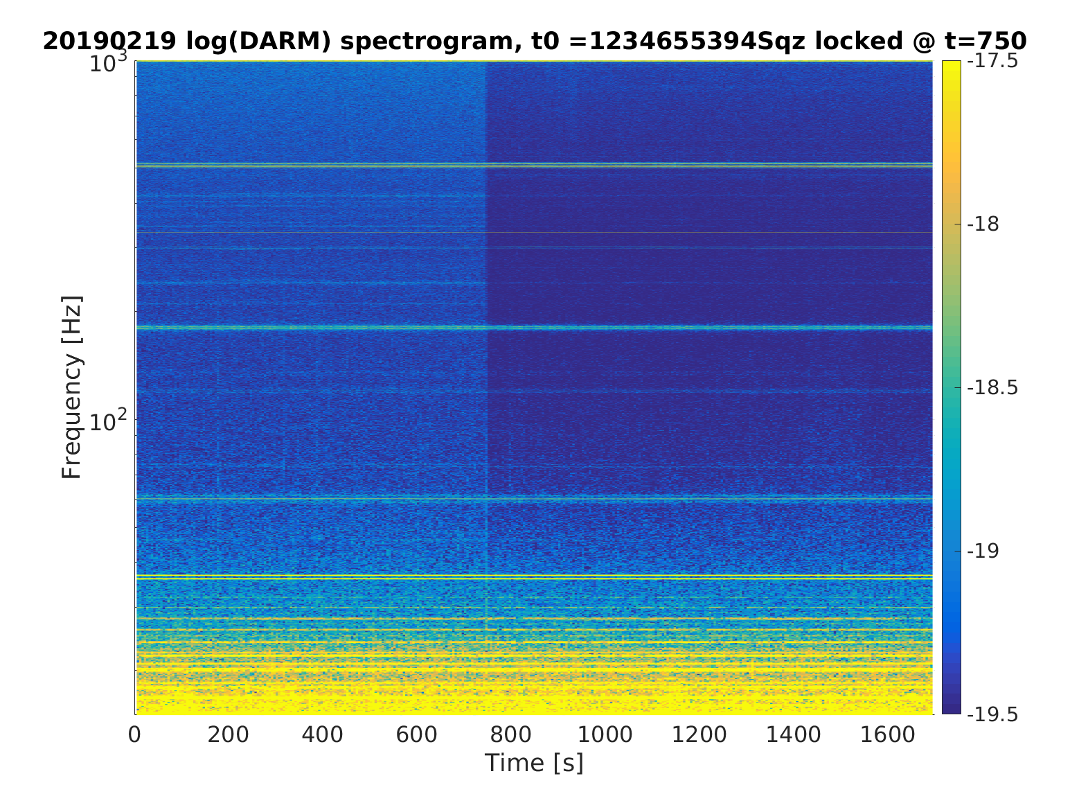
When the beam diverter was opened to inject squeezing this evening we noticed that the 20-29Hz DARM BLRMS got noisier. I made a quick spectrogram and it looks like there are lines at roughly 24 Hz, 26 Hz, 30 Hz, and 32 Hz that show up when the beam diverter is opened. In the first attachment the beam diverter is opened at ~t=500s. Note that the squeezing angle was unlocked for the duration of this spectrogram.
The second attachment shows the spectrogram up to 1kHz when the squeezing angle was locked, showing satisfying broadband noise improvement upon locking.
Since apparently you gain one dB at each attempt, you just need to do squeezing injection one more time! :-D
Great progress, well done!
Very cool! Take that, infinite sea of noisy energy.
Do you see a time dependence or fluctuation in the RF3-Q? That might indicate that some of the loss is time-dependent (and will be removable by controls).
One pedantic note about your plot. It looks like your X-axis is really the nonlinear gain you quote above. Since the seed field you use to measure NLG is injected through a different mirror, it is not measuring the parametric gain that the vacuum is squeezed by, so I wouldn't use that label. The vacuum is a reflection from the cavity M1, not transmission between M2 and M1 like the diagnostics fields. If you do use that label, then you should pass the NLG through the NLG->dbs formula and plot vs. "generated squeezing".
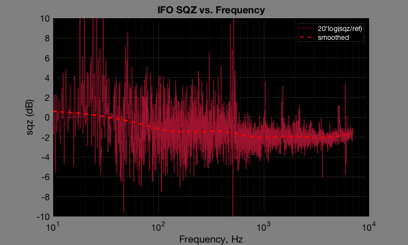
Attached frequency dependent sqz level plot. I divided squeezed spectrum by the reference, turned that into dB and then plot the average (using smooth() function in matlab).

We were moving CLF phase pretty much the whole time we were squeezing so I can't say there is or there isn't a time dependent Qmon fluctuation.
J. Kissel, E. Goetz Since we haven't had a number to reflect the answer to perennial question "what's the status of the calibration?" in what *feels* like a long time (the last time we were able to quantify its badness was on on 2019-01-31, based on a measurement from 2019-01-18, see LHO:46723), I've been given time to take a PCAL to DELTAL_EXTERNAL sweep today. As a result of successfully gathering this sweep, I was able to -- offline -- correct all* systematic errors in the DELTAL_EXTERNAL ASD, and compute the range -- at one time -- 120 seconds of data starting at 2019-02-19 23:00 UTC. This time was a thermally stabilized, and otherwise undisturbed with all calibration lines on. The plot aide is attached, but the sweep indicated a frequency dependent systematic error with excursions as high as 20%. The conclusion is that DELTAL_EXTERNAL is under-reporting H1's range by (85.45 - 75.35)/85.45 = 0.1182 ~ 12%. *This is, of course, assuming PCAL is a perfect calibrator. It should be damn close as the PCAL Y recently had a tune-up and remeasure of its force coefficient -- see LHO:46695, but I only balk a bit because of the recent evidence for clipping -- see LHO:46847. While I can't specifically attribute the systematic error to any one thing, I can point you to an aLOG in which I describe the current (well -- 2 weeks ago now) status of what I believe I need to do in order to correctly *remove* this systematic error: LHO:46806. Sadly, because of the snow-blizzard and lack of person power, I haven't made much *tangible* progress at all. The data lives here: (1) 2019-02-19_H1_PCAL2DARM_TF_5t1100Hz_8min.xml [Contains both DELTAL / PCAL and C/(1+G) measurements] (2) 2019-02-19_H1DARM_OLGTF_5to1100Hz_20min.xml [Contains both G and 1/(1+G) measurements] (3) 2019-02-19_H1_OMCDCPDSUM_to_DARMIN1.xml [Contains information to turn DARM IN1 counts roughly into DCPD SUM Current in "mA"] Note -- I only *need* needed measurement (1), but I was generously given a bit more time. I've worked my way through using Evan's command line function, /ligo/svncommon/CalSVN/aligocalibration/trunk/Common/pyDARM/correct_bns_range.py It required I create a new loop model, /ligo/svncommon/CalSVN/aligocalibration/trunk/Runs/O3/H1/params modelparams_H1_20190219.py The exact command line sequence I used for the function is python3.6 correct_bns_range.py --run='O3' --IFO='H1' --GPSstart='1234652418' --GPSend='1234652538' --PCAL2DARMTF='/ligo/svncommon/CalSVN/aligocalibration/trunk/Runs/O3/H1/Measurements/FullIFOSensingTFs/2019-02-19_H1_PCAL2DARMTF_A_PCALYRX_B_DELTALEXT_tf.txt' --PCAL2DARMCOH='/ligo/svncommon/CalSVN/aligocalibration/trunk/Runs/O3/H1/Measurements/FullIFOSensingTFs/2019-02-19_H1_PCAL2DARMTF_A_PCALYRX_B_DELTALEXT_coh.txt' --DARMmodelfile='modelparams_H1_20190219' --modelFunction='modelPars'
The BNS range corrected strain data can be found attached here, and committed to
/ligo/svncommon/CalSVN/aligocalibration/trunk/Runs/O3/H1/Results/FullIFOSensingTFs/
2019-02-19_H1_sensingFunction_BNSRangeCorrection.txt
Processed the sensing function. Added more points at low frequency to hope resolve the detuning parameters. More details to come.
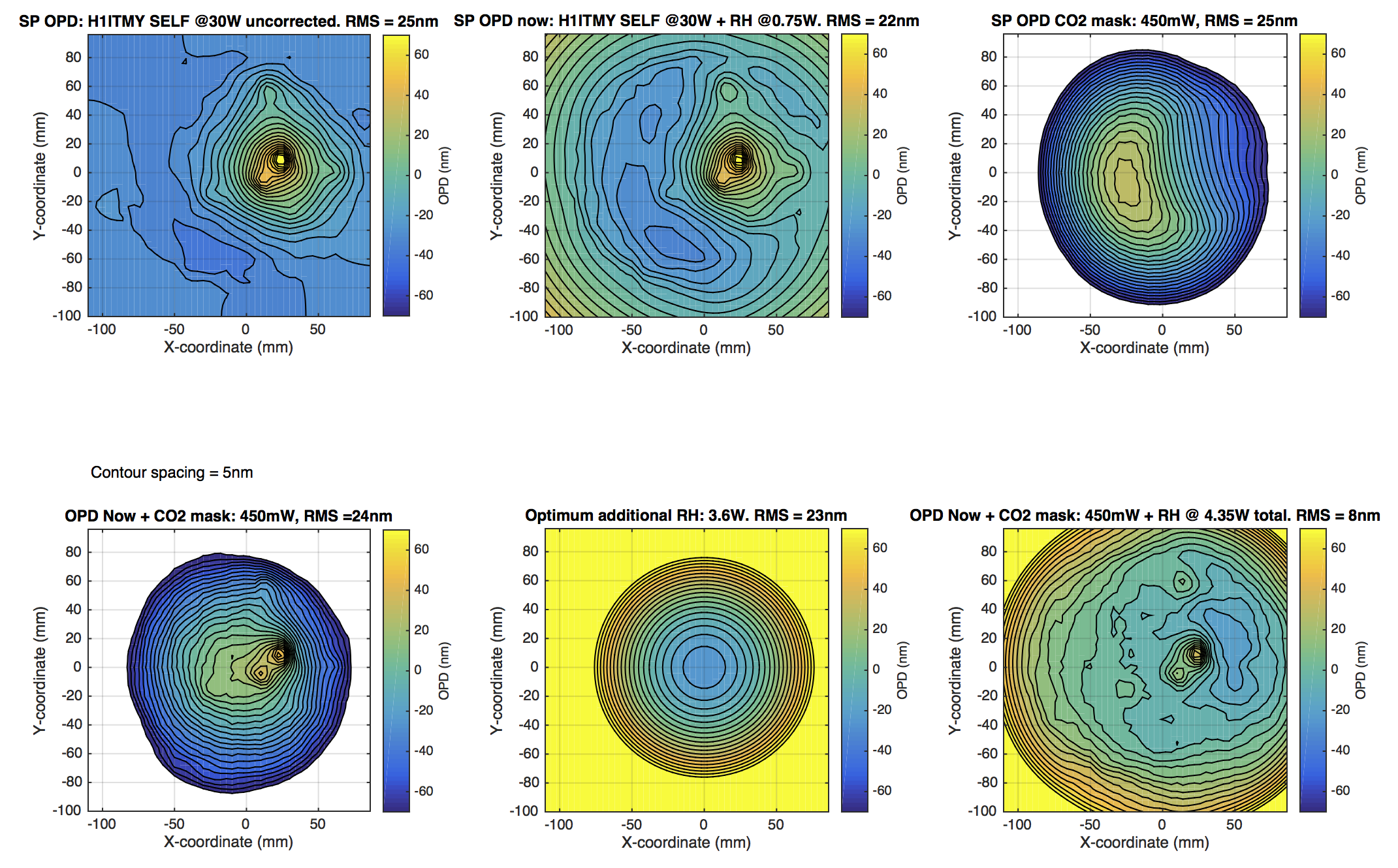
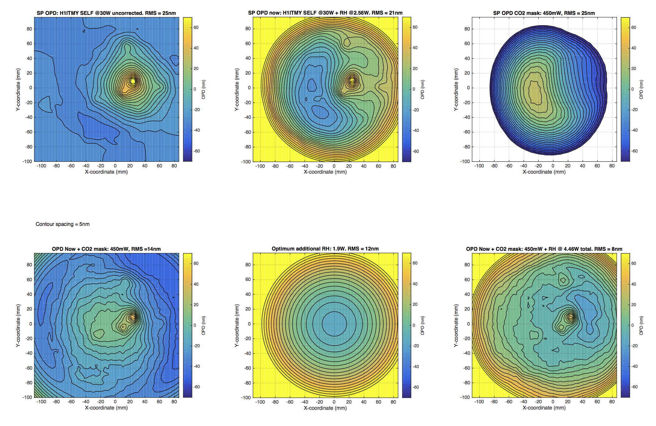
The following is a short summary of an approach to commissioning the H1 ITMY CO2 mask, D1900030. The purpose of the mask is to reduce the scattering of sidebands into higher order spatial modes. However, when the mask is simply applied by itself, it creates a strong positive quadratic lens. A combination of the ITMY RH, ITMX CO2 central heating and ITMX RH must be used to minimize the overall effect of the COMMON & DIFFERENTIAL MICH lenses and the COMMON and DIFFERENTIAL ITM curvatures.
The application of the mask is illustrated in the attached PDFs. An example of the application is shown here:
Note that (a) the color scales have been set to the same level [-70, 70]nm for comparison between different plots [so there is some saturation in some of the plots], (b) contours are set to 5nm spacing in all plots, (c) DC levels have been subtracted from each image so that the Gaussian weighted mean value is 0nm.

Once this step has been applied, the ITMY substrate lens should be same as it currently is. This will maintain the COMMON and DIFFERENTIAL MICH lenses. However, the application of ITMY RH will change the ITMY ROC and, hence, the COMMON and DIFF ITM ROC will need to be corrected. Which will be dealt with in step 2.
The attached PDFs show the effect for differing CO2 powers ranging from 50mW to 750mW. The minimum RMS OPD is achieved around 450mW.
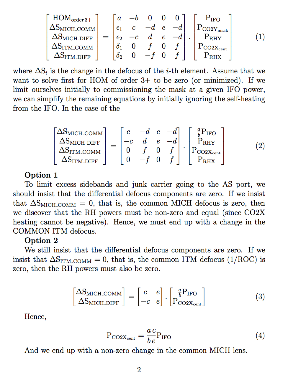
Working on the full matrix description of this: 4 TCS actuators > 4 DOF (COMM/DIFF MICH, COMM/DIFF ITM ROC).
Somewhat crude matrix analysis of actuation strategies. The effect of interferometer power and the CO2 mask can be seen below. Any actuation strategy that employs this mask will enforce a change in either the COMMON ITM ROC/DEFOCUS and/or the COMMON MICH DEFOCUS.

I'm working on plotting the time evolution of the RMS value of the OPD once the mask is added. However, as a rough guide (based on (a) some provisional simulations, (b) basic thermal diffusivity calculations), the thermal time constant of the mask is approximately 40 minutes. This means that the majority of the effect the mask should manifest on this time scale.
Note: this excludes the time constant associated with the RH
I just discovered that the code used to generate the wavefronts was using the ITMX RH power (~0.78W) rather than the ITMY RH (~2.56W). I'll need to regenerate these plots with the correct RH power.
Here is the updated mask application based on 2.56W into ITMY RH.